
Chapter 5. Quantum Chemistry
Propagation of Electronic Structure on a GPU
Jacek Jakowski, Stephan Irle and Keiji Morokuma
In direct molecular dynamics (MD) methods the nuclei are moving classically, using Newton's equations, on the quantum mechanical potential energy surface obtained from electronic structure calculations
[1]
[2]
and
[3]
. This potential energy surface is recalculated every time the nuclei change their positions, or as the chemists and physicists say, it is calculated “on the fly.” In order to compute a meaningful trajectory one has to perform several thousands of electronic structure calculations. The electronic structure is a central quantity that contains the information about forces acting on nuclei as well as the energy and chemical reactivity of molecules. The determination of electronic structure and its changes as the nuclei are moving is the central problem of direct dynamics methods
[4]
. In the typical Born-Oppenheimer MD approaches, the electronic structure is obtained through diagonalization of the Hamiltonian matrix from which the molecular orbitals are found and all chemically interesting properties are derived. This is in contrast to Car-Parrinello MD (CPMD) approaches where molecular orbitals (MOs) are propagated simultaneously with the nuclei, using Lagrangean dynamics in conjunction with a fictitious MO mass
[3]
. A severe limitation of CPMD is that the orbital occupations are fixed throughout the dynamics. Liouville-von Neumann MD (LvNMD)
[5]
solves the time-dependent Schrodinger equation for the time propagation of the wavefunction and allows fractional occupation numbers for MOs, which are important to describe mixed quantum states and metallic systems. We show in this chapter (a) how the electronic structure can be propagated without diagonalization in the LvNMD approach, (b) how to cast our problem for GPU in such a way as to utilize the existing pieces of GPU codes, and (c) how to integrate GPU code written in C/CUDA with the main Fortran program. Our implementation combines Fortran with non-thunking CUBLAS (matrix multiplications) and direct CUDA kernels.
5.1. Problem Statement
5.1.1. Background
The physical model for the direct molecular dynamics described here contains nuclei and electrons. All nuclei are treated classically as point particles with mass and electric charge. All electrons are treated quantum mechanically within the so-called independent particle model. The
density functional theories
,
Hartree-Fock
and
tight-binding methods
, are independent particle model methods. In the independent
particle model the interaction between electrons is treated in an average way. Each electron can feel only an average field from all other electrons. The interaction between electrons is described by the Fock operator matrix. The Fock operator also contains other information such as the kinetic energy of electrons and the interactions of electrons with nuclei. The determination of electronic structure evolution as the nuclei are moving is the central problem of direct dynamics methods
[4]
.
Electronic structure in quantum chemical applications can be represented by a wave function or equivalently by a density matrix. To construct an electronic wave function or a density matrix, one starts by choosing a physically meaningful set of basis functions
 (e.g., Gaussians centered on atoms or plane waves). The behavior of each electron is described through molecular orbitals,
 , which are linear combinations of basis function
 where
where
 runs over all basis functions and
 labels different molecular orbitals. The number
 of basis functions used corresponds to the size of the system measured in atoms or electrons. The coefficients
 are typically obtained from diagonalization of the Fock operator. The
 electronic wavefunction can be constructed as a determinant (or combination thereof) build of occupied molecular orbitals. In an equivalent density matrix representation, instead of using
 coefficients, one can use an M × M matrix to directly describe electronic structure. The relation between molecular orbital coefficients
 and density matrix elements
 is
is
 where
where
 denotes a complex conjugation of
 and
and
 is an occupation number (between 0 and 1).
(5.1)
(5.2)
Overview of Direct Dynamics Theory
In direct molecular dynamics, the positions of nuclei are changing with time and the electronic structure adjusts following the time-dependent Schroedinger equation (TDSE). Time dependence of electronic structure is often neglected, and instead, the time-independent Schroedinger equation is solved. This leads to the so-called Born-Oppenheimer approximation
[1]
and
[2]
. In the density matrix representation of electronic structure, the TDSE becomes the von Neumann equation
 where
where
 and
and
 denote the time-dependent density and Fock operator matrices, respectively
[5]
. In principle, both
denote the time-dependent density and Fock operator matrices, respectively
[5]
. In principle, both
 and
and
 are complex square matrices of size
 . The propagation of density matrix described by
Eq. 5.3
is an initial value problem subject to initial density matrix
. The propagation of density matrix described by
Eq. 5.3
is an initial value problem subject to initial density matrix
 . The solution is obtained by time integration of
Eq. 5.3
on some discretized time interval
. The solution is obtained by time integration of
Eq. 5.3
on some discretized time interval
 with the
 sampling time step. Starting from time
 and initial density
 we find the density
 from
from
 as
as
 where
where
 , and
, and
 is the Fock operator, and
 is a quantum mechanical time-evolution operator
 Here, we approximate the time-evolution operator as
 where
where
 is taken as an average Fock operator on the time interval
 and
and
 .
.
(5.3)
(5.4)
(5.5)
Now, to obtain the propagated density matrix
 from
from
 , one can (a.) diagonalize
 to obtain the exponential time evolution operator,
 , which is then directly applied in
Eq. 5.4
, or (b.) apply the Baker-Campbell-Hausdorf (BCH) expansion and thus avoid diagonalization. Here, we focus on the latter approach. The final expression for the time evolution of density matrix from
, which is then directly applied in
Eq. 5.4
, or (b.) apply the Baker-Campbell-Hausdorf (BCH) expansion and thus avoid diagonalization. Here, we focus on the latter approach. The final expression for the time evolution of density matrix from
 to
to
 is
is
 where = AB-BA. To propagate the density matrix from time
 to
to
 , one must apply the propagation
 described by
Eq. 5.6
or by
Eq. 5.4
repeated
described by
Eq. 5.6
or by
Eq. 5.4
repeated
 times.
(5.6)
Problem Statement
In this chapter we show that the algorithm based on diagonalization and which also maps poorly to GPU architecture can be replaced by an alternative approach that is based on matrix-matrix multiplication that maps well to GPU architectures. We also show how our density matrix propagation code for GPUs is merged with a main Fortran program. Computational chemists, especially those interested in quantum chemistry, often face the challenge of dealing with large legacy codes written in Fortran. For example, a quantum chemistry package Gaussian was initially released in 1970. Its latest release, Gaussian 09, has 1.5 million lines of Fortran code developed by several authors
[6]
. It is a formidable challenge to use the features provided in such programs in conjunction with GPU accelerators. Finally, for performance reasons, the authors’ philosophy is to use existing efficient libraries whenever possible. This allows to offload the optimization effort to the library vendor. Several efforts are now ongoing toward developing such efficient GPU libraries
[7]
[8]
and
[9]
. Although these libraries
[8]
and
[9]
are not yet fully functional, we anticipate that their role in programmming will be increasing.
In this chapter we discuss the GPU implementation of density matrix propagation via
Eq. 5.6
. We show (a.) how the electronic structure can be propagated without diagonalization, (b.) how to cast our problem for GPUs in such a way as to utilize the existing pieces of GPU codes, and (c.) how to integrate GPU code written in C/CUDA with the main Fortran program. Our implementation combines Fortran with non-thunking CUBLAS (matrix multiplications) and direct CUDA kernels.
5.2. Core Technology and Algorithm
5.2.1. Discussion of Technology
The current implementation combines Fortran with C and CUDA. The main program and initialization of the dynamics is written in Fortran. For each time step of MD (Molecular Dynamics) the Fock matrix
is evaluated on the CPU and transferred to GPU memory. The density matrix is then propagated on the GPU according to
Eq. 5.6
and the result is transferred back to CPU for analysis. Thus, two memory transfers between CPU and GPU are performed for each MD time step.
Figure 5.1
shows a schematic execution chain of the program for the two consecutive MD time steps.
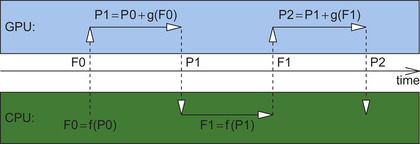 |
| Figure 5.1
Main program execution flow for the two consecutive time steps of Liouville-von Neumann molecular dynamics. Operations performed on GPUs (propagation of density matrix) are schematically shown in the light gray box. Operations performed on CPUs (evaluation of Fock matrix and update of nuclei positions) are schematically shown in the dark gray box. Vertical arrows represent transfers of Fock (F) from CPU to GPU and transfer of density matrix (P) in the opposite direction. The MD time is shown as x-axis between the GPU and CPU boxes.
|
We analyzed the computational of the density matrix propagation for various GPU programming models. We tested a PGI Accelerator directives-based Open-MP-like programming model
[10]
and CUDA with the CUBLAS library
[7]
. The final GPU code combines matrix multiplication from the CUBLAS library with the CUDA kernel for the matrix transpose. The CUDA transpose kernel is a simple implementation optimized for shared memory access, and it uses a thread block size 16 × 16 (see
CUDA SDK Code Samples
[11]
). The discussion describing the chosen programming model is presented in Section 3. We compare the simulation results on the GPU with the best CPU implementation optimized by us.
The CPU host code that directly calls kernels on the device is written in C/CUDA. Wrappers written in C are used to bind the main Fortran code with CUDA code. The hierarchy of code access to the GPU device from Fortran is shown in
Figure 5.2
.
Figure 5.4
shows the code sample that describes the GPU access from Fortran.
| Figure 5.2
Schematic description of access to a GPU device from Fortran code. The dark gray boxes denote code compilable with the standard Fortran compiler. The light gray box denotes code written in C/CUDA.
|
Discussion of Algorithm
The overview of the algorithm for the density matrix propagation on the GPU from time
 to time
 is presented in
Figure 5.3
.
is presented in
Figure 5.3
.
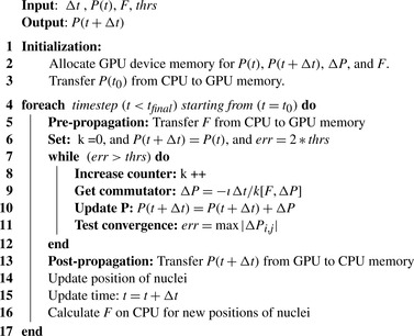 |
| Figure 5.3
Density matrix propagation via
Eq. 5.6
. The evaluation of commutator expansion terms is suspended when the convergence is smaller than the threshold
thrs
.aaa
|
 |
| Figure 5.4
Code sample for GPU access from Fortran to CUDA. Notice that the “GPU pointer”
devA
can be passed from
transp.F
to the calling subroutine as an integer.
|
Here are some details and tricks used in the final implementation:
(a) The algorithm requires an allocation of the memory for
 (size of real
 ), initial and final
 (size of complex
 ), a matrix for the intermediate result of commutator
 (size of complex
 ), and an additional scratch array the same size as
 (size of real
 ).
).
The expansion in
Eq. 5.6
represents a nested commutator. Each higher-order commutator can be obtained recursively from the previous one as
 for
for
 0 and
0 and
 .
.
(5.7)
Each commutator term can be treated as an update to the density matrix
 Thus, at any given time, it is only necessary to store
 ,
,
 ,
,
 and
and
 matrices.
(5.8)
(b) The commutator expansion in
Eq. 5.6
is truncated when the largest matrix element of
 is smaller than a preset threshold
 . We use threshold value
 . Sacrificing accuracy by using a lower threshold would allow the calculation to speed up.
(c) In the current electronic structure model (density functional tight-binding theory
[14]
and
[15]
), the imaginary part of the Fock operator vanishes. The Fock matrix depends only on the real component of the density matrix
[5]
. It is currently evaluated on the CPU and transferred to GPU memory. Matrix
 is real and symmetric. Matrices P and
 are complex and self-adjoint with the real part being a symmetric matrix (S) and the imaginary part being an antisymmetric matrix (A). Contrary to this, time evolution matrix
 is a general complex.
(d)
All complex quantities are stored and processed as separate, real, and imaginary matrices. For example, the real and imaginary components of hermitian matrix
 are stored as a separate symmetric matrix (S) and antisymmetric matrix (A).
 Separating real and imaginary components of complex matrices turned out to be beneficial for both efficiency and practical reasons. For example, to perform a matrix product operation between
 and
and
 , it is twice as cheap to perform two real matrix multiplications (as
 followed by
 ), than one matrix product between two complex matrices with the imaginary part of
 set to zero.
(5.9)
(e)
The basic quantity to be calculated repeatedly in
Eq. 5.6
is a matrix commutator
 . In principle, to evaluate commutator
 for general matrices
 and
and
 , one has to perform two matrix multiplications (
 and
and
 ). However, if
 and
and
 are symmetric or antisymmetric, then it is possible to evaluate
 as one matrix multiplication and one transpose. That is
 ,
,
 , and
, and
 . As we show in the next section of this chapter, the cost of a matrix transpose is significantly lower than the cost of matrix multiplication. We notice that in expression
 the
the
 matrix is symmetric (S) while
 is a sum of symmetric (S) and antisymmetric (A) components.
(f) All matrices are treated as super vectors of size M × M, which allows the utilization of level 1 BLAS routines
[12]
for scalar matrix operations.
5.3. The Key Insight on the Implementation—the Choice of Building Blocks
In the process of designing a new scientific computing method, one has to answer several questions in order to choose the best possible available building blocks for the program. What is the problem size that one wants to tackle? What is the expected scaling method with respect to the system size? What is the direct and relative cost of different code components in the program for a given problem size (this depends on scaling of the components)? What is the most expensive operation and how often is it used? Are there any preexisting libraries or codes that can be used as building blocks? How efficient are the libraries compared with intrinsic functions and compiler optimized codes? Is there any special structure or pattern to the data that would allow one to modify the algorithm to improve its efficiency? What is the outlook for further improvements or hardware changes? These questions are relevant for both CPU and GPU implementation. We are interested in having the best possible implementation on the CPU as well as the GPU.
The problem size we want to tackle, a quantum chemical simulation of carbon nano-nanomaterials for material science problems, ranges from a few hundred to several thousands of basis functions (see
Figure 5.5
). The basic operation in the program is the evaluation of the scaled commutator
 . This can be split into more “primitive” operations such as matrix-matrix multiplication, matrix addition/subtractions, and matrix-scalar product. The computational cost of the
first operation (matrix-matrix multiplication) scales cubically with the matrix size M. The cost of matrix-scalar multiplication and matrix-matrix addition/subtraction scales quadratically with
. This can be split into more “primitive” operations such as matrix-matrix multiplication, matrix addition/subtractions, and matrix-scalar product. The computational cost of the
first operation (matrix-matrix multiplication) scales cubically with the matrix size M. The cost of matrix-scalar multiplication and matrix-matrix addition/subtraction scales quadratically with
 .
.
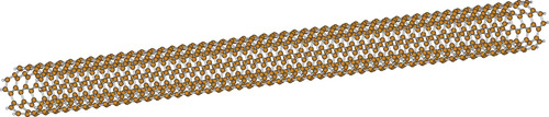 |
| Figure 5.5
Single-wall carbon nanotube of (5,5) type with hydrogen-terminated ends. The total number of atoms is 1010. The total number of basis functions for DFTB calculations is 3980. Carbon nanotubes and other carbon-based nanomaterials are very promising materials for the nanotechnology and materials science fields and are hoped to be used as molecular electronic wires in a new generation of electronic devices.
|
Matrix Multiplication
As was discussed in
Section 5.2
of this chapter, matrices
 and
and
 in the commutator expression
 can either be symmetric or antisymmetric for the physically meaningful cases. However, the product of symmetric and/or antisymmetric matrices is a general matrix, but its commutator reveals symmetry properties that can be exploited in the implementation. The commutator of matrices of the same type (both symmetric or both antisymmetric) is an antisymmetric matrix. The commutator of a symmetric matrix with an antisymmetric matrix is always a symmetric matrix. Furthermore, once the matrix product
 is known, then the second product can be replaced by its transpose. Specific questions we want to answer are: What is the computational cost of various versions of matrix-matrix multiplications on CPU and on GPU? Is it better to use a matrix transpose or matrix multiplication? The product of two symmetric or general matrices can use specialized routines from BLAS
[12]
. How expensive is the cost of multiplication for two symmetric [
ssymm()
] versus the product of two general matrices [
sgemm()
]?
is known, then the second product can be replaced by its transpose. Specific questions we want to answer are: What is the computational cost of various versions of matrix-matrix multiplications on CPU and on GPU? Is it better to use a matrix transpose or matrix multiplication? The product of two symmetric or general matrices can use specialized routines from BLAS
[12]
. How expensive is the cost of multiplication for two symmetric [
ssymm()
] versus the product of two general matrices [
sgemm()
]?
First, let us compare the performance of different versions of general matrix multiplication on a CPU and on a GPU. For a CPU, one can test compiler optimization, intrinsic Fortran 90 matrix multiplication, and various versions of BLAS. For the matrix multiplication on a GPU, we tested CUBLAS, a handmade CUDA kernel, and PGI accelerator directives. Some of our test results comparing different versions of general matrix-matrix multiplication are shown in the
Table 5.1
. Next, we compared the symmetric and general matrix multiplication in
Table 5.3
. The GPU calculations were performed on a Tesla C1060 with the PGI F90 compiler. All CPU calculations were performed on dual Quad Core Intel Xeon 2.5 GHz Harpertown E5420 (em64t) machine with 16 GB RAM.
The conclusion of our matrix multiplication tests are the following. The best results for the CPU were obtained with Intel's MKL routines
[13]
. Matrix multiplication with CUBLAS led to superior matrix multiplication results on the GPU. No performance gain was observed by using symmetric versions of matrix multiplication (ssymm()
) as compared with the general case (sgemm()
).
Table 5.2
compares CUBLAS matrix multiplication for a matrix size as a multiple of 1000 with slightly larger matrices of size equal to multiples of 64. This shows that padding matrices with zero to match the size equal to multiplies of 64 can result in better memory access and decrease the total calculation time by up to 50% in some cases. Overall, we conclude that for CPU implementation one should use multithreaded MKL, while the GPU implementation should be based on CUBLAS matrix multiplication.
Transpose and Other Operations
Finally, we compared the relative cost of matrix multiplication with matrix transpose and other matrix operations that we encounter in our algorithm. The results are presented in
Table 5.3
. Our tests show that the cost of matrix transpose amounts to no more than a few percent when compared with matrix multiplication. Also, the cost of other matrix operations is very small in comparison to the cost of matrix multiplication.
Based on our knowledge of the properties of matrices, the analysis of the density matrix algorithm, and on the tests we performed, we conclude, thus, that the optimal implementation of density matrix propagation should follow these recommendations:
1. It is beneficial to split the complex
 matrix into real and imaginary matrices and then perform two real matrix multiplications of real
 with real and imaginary components of
 . Using this procedure for the product of real
 with complex
 saves half of the time.
3. While using CUBLAS matrix multiplication, it is very beneficial to pad matrices so that their leading dimension is a multiple of 64.
4. There is not much gain by using symmetric matrix multiplication routines (ssymm()
) rather than general ones (sgemm()
).
5. The cost of computing the transpose is very small compared with the cost of matrix multiplication. Also the cost of matrix-scalar multiplication (matrix scaling by
sscal()
) and other matrix operations that can be mapped to level 1 BLAS routines is much smaller than the matrix-matrix multiplication. Thus, it is of secondary importance which version of transpose or of any other operation is used. However, using BLAS
[12]
routines guarantees that the code is independent of the machine architecture and the cost of optimization is placed on the library vendor.
6. The optimal implementation of the matrix commutator should use one matrix-matrix multiplication followed by one transpose, rather than two matrix multiplications.
Following the conclusion of the discussion in
5.2
and
5.3
, we implemented and tested both CPU and GPU versions of density matrix propagation. For the CPU implementation we used Intel's MKL as this leads to the best performance on the CPU. For the final evaluation we performed three sets of tests. First, we compared the performance of our GPU implementation of
Eq. 5.6
with the analogous CPU implementation based on MKL for random
 and
and
 . In the second test, we compared the GPU implementation with CPU propagation based on direct evaluation of the time-evolution operator through diagonalization of the Fock operator. For these tests we also used random
 and
and
 matrices. In the final real case test, we compared the timing for density matrix propagation on the GPU for a carbon nanotube containing 1010 atoms (
 ). The structure of a carbon nanotube for which we performed the test is shown in
Figure 5.5
. The corresponding number of basis functions is 3980 for
). The structure of a carbon nanotube for which we performed the test is shown in
Figure 5.5
. The corresponding number of basis functions is 3980 for
 and
and
 . The matrices for the GPU simulation were padded with zeros to match the size 4032, which is the nearest multiple of 64.
Fock and Density Matrices
For the timing tests we generated random Fock and density matricies of various sizes ranging from M = 500 to M = 4096. To make the density matrix more physical, we scaled the density matrix to make its trace equal to M/2 (the trace of a density matrix is equal to the number of electrons in the molecular system). For a similar reason, we multiplied each randomly generated matrix element of the Fock operator by
 . The chosen values were consistent with our previous simulation of carbon-based nanomaterials performed at the DFTB level of theory
[14]
and
[15]
. We also chose the value of the threshold for the convergence of the density matrix propagation (see 2.ii) given by
Eq. 5.6
to be equal to
. The chosen values were consistent with our previous simulation of carbon-based nanomaterials performed at the DFTB level of theory
[14]
and
[15]
. We also chose the value of the threshold for the convergence of the density matrix propagation (see 2.ii) given by
Eq. 5.6
to be equal to
 . We observed that our commutator expansion converged after around 20 commutator iterations. This, again, was consistent with our previous simulations performed for carbon-based nanomaterials
[5]
. Thus, we believe that the current tests for random matrices represents the real simulations of carbon nanomaterials well. For the real case test we used armchair (5,5) single-wall carbon nanotubes as well (see
Figure 5.5
). The test system contained a total of 1010 atoms, including 990 carbons and 20 terminating hydrogens. For the carbon nanotube simulation, we used DFTB theory. The corresponding number of basis functions in DFTB for
. We observed that our commutator expansion converged after around 20 commutator iterations. This, again, was consistent with our previous simulations performed for carbon-based nanomaterials
[5]
. Thus, we believe that the current tests for random matrices represents the real simulations of carbon nanomaterials well. For the real case test we used armchair (5,5) single-wall carbon nanotubes as well (see
Figure 5.5
). The test system contained a total of 1010 atoms, including 990 carbons and 20 terminating hydrogens. For the carbon nanotube simulation, we used DFTB theory. The corresponding number of basis functions in DFTB for
 and
and
 was 3980. The matrices for the GPU simulation were padded with zeros to match a multiple of 64. Thus, the size of
 and
and
 for GPU simulations was 4032. We did not use padding of
 and
and
 for the CPU.
Hardware
The CPU tests were performed on a machine with 16 GB RAM and two quad core Intel Xeon model E5420 Harpertown processors with a 2.5 GHz clockspeed and 24 MB L2 cache (6 MB per core pair). Our CPU code used the multithreaded Math Kernel Library (MKL)
[13]
. Thus, for the CPU tests, we propagated the density matrix in parallel with up to eight cores. Consequently, our CPU code could run in parallel with eight cores. For the GPU tests we used a Tesla C1060 processor and the 2.3 version of the CUDA SDK. The GPU processor C1060 contained 240 single-precision (SP) cores and 30 double-precision (DP) cores clocked at 1.3 GHz. The number of cores had a significant impact on the performance. To see this effect we performed tests for both single-precision (SP) and double-precision (DP) implementations on the GPU and we compared them with analogous CPU implementations.
Discussion
Table 5.4
compares the GPU implementation for the density matrix propagation with the analogous CPU implementation based on multithreaded MKL
[13]
. In
Table 5.5
we compare results
on the GPU obtained for the BCH algorithm with the CPU results for the single and multithreaded diagonalization (dsyev()
via MKL) algorithm. As can be seen in
Table 5.4
and
Table 5.5
, the density matrix propagation scales cubically with the system size. That is, as the system size (matrix size) increases twice (for example, from 1024 to 2048) we observe a
 times increase in computation time. This is
inherently related to the fact that the computing engine for the density matrix propagation relies heavily on the dense matrix-matrix multiplication. The same is true for diagonalization.
times increase in computation time. This is
inherently related to the fact that the computing engine for the density matrix propagation relies heavily on the dense matrix-matrix multiplication. The same is true for diagonalization.
We observe an eightfold speedup when using eight MKL threads as compared with a single MKL thread. For example, for
 in
Table 5.4
the CPU time spent on single-threaded MKL calculation is 884 seconds while the same calculation with eight threads takes 111 seconds. When switching from single to double precision on the GPU, we observe about 4–5 times degradation in performance. This roughly corresponds to the 8 to 1 ratio of the number of single- over double-precision cores in the C1060. Our results suggest that the BCH algorithm for density matrix propagation has a strong scaling. This is a very promising indicator since current trends in computer architectures (for both CPU and GPU) is to provide more cores per unit. NVIDIA's Fermi, a new generation GPU, will have a significantly larger number of cores as compared with the Tesla C1060, and we expect a significant speedup of our BCH code on Fermi.
in
Table 5.4
the CPU time spent on single-threaded MKL calculation is 884 seconds while the same calculation with eight threads takes 111 seconds. When switching from single to double precision on the GPU, we observe about 4–5 times degradation in performance. This roughly corresponds to the 8 to 1 ratio of the number of single- over double-precision cores in the C1060. Our results suggest that the BCH algorithm for density matrix propagation has a strong scaling. This is a very promising indicator since current trends in computer architectures (for both CPU and GPU) is to provide more cores per unit. NVIDIA's Fermi, a new generation GPU, will have a significantly larger number of cores as compared with the Tesla C1060, and we expect a significant speedup of our BCH code on Fermi.
In the case of the BCH algorithm, the computational cost depends on a time step used in molecular dynamics (see
Table 5.5
). For the larger time steps the more terms of commutator expansion is required to achieve the convergence for a given threshold. Here, we use convergence threshold value
 . Thus, overall cost and accuracy in the BCH algorithm can be controlled by the time step and BCH convergence threshold. The cost for the diagonalization-based algorithm is independent of the time step and accuracy versus cost cannot be controlled.
For the final test we propagated the density matrix in a large carbon nanotube (see
Figure 5.5
) at the DFTB level of theory. The corresponding size of
 and
and
 matrices is 3980. For the GPU we increased the size to the nearest multiple of 64 larger than 3980. The computational cost amounts to 10 seconds and 49 seconds for single- and double-precision propagation of the density matrix on the GPU, respectively. Similarly, the CPU time for the propagation of the density matrix via MKL diagonalization is 70 seconds.
Overall, for the double-precision implementations on GPU compared with the CPU we obtain a twofold speedup for 8-thread MKL execution and nine times speedup for the single-thread MKL execution. For the analogous single-precision implementations we obtain a speedup of five times with respect to the 8-thread MKL execution on the CPU and 20 times the speedup for a single-thread MKL run. Our results show that the relative (CPU vs. GPU) computational cost is in good agreement with an estimate from the hardware specification. For the single-precision implementation one can expect that 240 GPU cores of 1.3 GHz, as compared with eight CPU cores clocked at 2.5 GHz, would lead to about 16 times the speedup [(240 cores * 1.3 GHz)/(8 cores * 2.5 GHz)]. Similarly, for double precision one can expect about a twofold speedup [(30 cores * 1.3 GHz)/(8 cores * 2.5 GHz)].
Benefits
The benefits of current implementation are
• Our GPU algorithm shows a reasonable improvement over the CPU implementation and a promising strong scaling;
• The code and GPU subroutines can easily be connected with any Fortran code due to the top layer wrappers Fortran-to-C inferface. This is important considering the fact that a large portion of computational chemistry software is legacy code written in Fortran;
• The propagation scheme is general and does not depend on the specific level of electronic structure used. It can be used with Hartree-Fock, density functional, or tight-binding theories. The general
modular character allows it to connect with any electronic structure method that can provide Fock evaluation;
• The Liouville-von Neumann propagation scheme
[5]
goes beyond the Born-Oppenheimer approximation.
5.5. Conclusions and Future Directions
Summary
We described our effort to adapt our quantum dynamics algorithm for the propagation of electronic density matrices on GPU. We showed how the Liouville-von Neumann algorithm can be redesigned to efficiently use vendor-provided library routines in combination with direct CUDA kernels. We discussed the efficiency and computational costs of various components involved that are present in the algorithm. Several benchmark results were shown and the final test simulations were performed for a carbon nanotube containing 1010 atoms, using the DFTB level of theory for electronic structure. Finally, we demonstrated that the GPU code based on a combination of CUDA kernels and CUBLAS routines can be integrated with a main Fortran code.
Here is the summary of the path we followed and the lessons we learned:
• Analyze the theoretical scaling of the algorithm and of its major components. Analyze the computation of various building blocks for the target problem size.
• Focus on the most expensive part (building block) of the algorithm. Use existing efficient libraries if possible. It is generally cheaper and more effective to use existing libraries than to optimize the code by hand.
• If the most expensive building blocks do not exist yet in the form of the efficient library and if no GPU library exists, then focus on the optimization of CUDA code.
Future Directions
We presented our experimental implementation of electronic structure propagation on GPUs. We plan to use this method for the material science simulations. In our future development we will focus on (a) moving the formation of the Fock matrix from the CPU to GPU, (b) adapting the algorithm for multi GPUs, and (c) exploiting sparsity of matrices.
Acknowledgments
The support for this project is provided by the National Science Foundation (grant No. ARRA-NSF-EPS-0919436). NICS computational resources are gratefully acknowledged. We would like to acknowledge the donation of equipment by NVIDIA within the Professor Partnership Program to K.M. J.J. would like to thank Jack Wells for the inspiring discussions. K.M. acknowledges support of AFSOR grants (FA9550-07-1-0395 and FA9550-10-1-030). S.I. acknowledges support by the Program for Improvement of Research Environment for Young Researchers from Special Coordination Funds for Promoting Science and Technology (SCF) commissioned by the Ministry of Education, Culture, Sports, Science and Technology (MEXT) of Japan.
[1]
W.K. Hase, K. Song, M.S. Gordon,
Direct dynamics simulations
,
Comput. Sci. Eng.
5
(4
) (2003
)
36
–
44
.
[2]
D. Marx, J. Hutter,
Ab initio molecular dynamics: theory and implementation
,
In: (Editor: J. Grotendorst)
Winterschool, Julich, Germany, 21–25 February 2000
.
Modern Methods and Algorithms of Quantum Chemistry Proceedings
,
1
(2000
)
John van Neumann Institute fur Computing
, pp.
301
–
449
.
[3]
R. Car, M. Parinello,
Unified approach for molecular dynamics and density-functional theory
,
Phys. Rev. Lett.
55
(22
) (1985
)
2471
–
2474
.
[4]
G. Fleming, M. Ratner, Directing Matter and Energy: Five Challenges for Science and the Imagination, A Report from the Basic Energy Sciences Advisory Committee, US Dept. of Energy,
http://www.sc.doe.gov/bes/reports/abstracts.html#GC
, 2007 (accessed on July 2010).
[5]
J. Jakowski, K. Morokuma,
Liouville-von Neumann molecular dynamics
,
J. Chem. Phys.
130
(2009
)
224106
.
[6]
M.J. Frisch, G.W. Trucks, H.B. Schlegel, G.E. Scuseria, M.A. Robb, J.R. Cheeseman,
Gaussian 09, Revision A.02
. (2010
)
Gaussian, Inc.
,
Wallingford, CT
.
[7]
CUDA CUBLAS Library,
http://developer.download.nvidia.com/compute/cuda/2_3/toolkit/docs/CUBLAS Library 2.3.pdf
.
[8]
CULA, A GPU-Accelerated Linear Algebra Library
, EM Photonics, Newark, DE,
http://www.culatools.com/features/
.
[9]
E. Agullo, J. Demmel, J. Dongarra, B. Hadri, J. Kurzak, J. Langou,
et al.
,
Numerical linear algebra on emerging architectures: the PLASMA and MAGMA projects
,
J. Phys.: Conf. Ser.
180
(2009
)
.
[10]
M. Wolfe, PGI Fortran & C Accelerator Programming Model, The Portland Group,
http://www.pgroup.com/lit/whitepapers/pgi_accel_prog_model_1.2.pdf
, 2010.
[11]
G. Reutsch, P. Micikevicius, Optimizing Matrix Transpose in CUDA, CUDA SDK Code Samples, NVIDIA, 2009.
[12]
L.S. Blackford, J. Demmel, J. Dongarra, I. Duff, S. Hammarling, G. Henry,
et al.
,
An updated set of basic linear algebra subprograms (BLAS)
,
ACM Trans. Math. Soft.
28
(2002
)
135
–
151
.
[13]
Intel Math Kernel Library 10.2,
http://software.intel.com/en-us/intel-mkl/
.
[14]
D. Porezag, Th. Frauenheim, Th. Köhler, G. Seifert, R. Kaschner,
Construction of tight-binding-like potentials on the basis of density-functional theory: application to carbon
,
Phys. Rev. B
51
(1995
)
12947
–
12957
.
[15]
M. Elstner, D. Porezag, G. Jungnickel, J. Elsner, M. Haugk, Th. Frauenheim,
et al.
,
Self-consistent-charge density-functional tight-binding method for simulations of complex materials properties
,
Phys. Rev. B
58
(1998
)
7260
–
7268
.
..................Content has been hidden....................
You can't read the all page of ebook, please click here login for view all page.