
Chapter 6. An Efficient CUDA Implementation of the Tree-Based Barnes Hut
n
-Body Algorithm
Martin Burtscher and Keshav Pingali
This chapter describes the first CUDA implementation of the classical Barnes Hut
n
-body algorithm that runs entirely on the GPU. Unlike most other CUDA programs, our code builds an
irregular
tree-based data structure and performs complex traversals on it. It consists of six GPU kernels. The kernels are optimized to minimize memory accesses and thread divergence and are fully parallelized within and across blocks. Our CUDA code takes 5.2 seconds to simulate one time step with 5,000,000 bodies on a 1.3 GHz Quadro FX 5800 GPU with 240 cores, which is 74 times faster than an optimized serial implementation running on a 2.53 GHz Xeon E5540 CPU.
6.1. Introduction, Problem Statement, and Context
The Barnes Hut force-calculation algorithm
[1]
is widely used in
 -body simulations such as modeling the motion of galaxies. It hierarchically decomposes the space around the bodies into successively smaller boxes, called cells, and computes summary information for the bodies contained in each cell, allowing the algorithm to quickly approximate the forces (e.g., gravitational, electric, or magnetic) that the
 bodies induce upon each other. The hierarchical decomposition is recorded in an octree, which is the three-dimensional equivalent of a binary tree. With
 bodies, the precise force calculation needs to evaluate
 interactions. The Barnes Hut algorithm reduces this complexity to
 and thus makes interesting problem sizes computationally tractable.
The Barnes Hut algorithm is challenging to implement efficiently in CUDA because (1) it repeatedly builds and traverses an irregular tree-based data structure, (2) it performs a lot of pointer-chasing memory operations, and (3) it is typically expressed recursively. Recursion is not supported by current GPUs, so we have to use iteration. Pointer-chasing codes execute many slow uncoalesced memory accesses. Our implementation combines load instructions, uses caching, and throttles threads to drastically reduce the number of main memory accesses; it also employs array-based techniques to enable some coalescing. Because traversing irregular data structures often results in thread divergence (i.e., detrimental loss of parallelism), we group similar work together to minimize divergence.
Our work shows that GPUs can be used to accelerate even irregular codes. It includes a number of new optimizations, as well as known ones, and demonstrates how to exploit some of the unique architectural features of GPUs in novel ways. For example, because the threads in a warp necessarily run in lockstep, we can have one thread fetch data from main memory and share the data with the other threads without the need for synchronization. Similarly, because barriers are implemented in hardware on GPUs and are therefore very fast, we have been able to use them to reduce wasted work and main memory accesses in a way that is impossible in current CPUs where barriers have to communicate through memory. Moreover, we exploit GPU-specific operations such as thread-voting functions to greatly improve performance and make use of fence instructions to implement lightweight synchronization without atomic operations.
The rest of this chapter is organized as follows:
Section 6.2
provides more detail on the Barnes Hut algorithm and how we mapped it to GPU kernels;
Section 6.3
describes the operation of each kernel with a focus on tuning; and
Section 6.4
evaluates the performance of our implementation, discusses limitations, and draws conclusions.
6.2. Core Methods
This section explains the Barnes Hut algorithm.
Figure 6.1
shows the high-level steps. Steps 1 through 6, that is, the body of the time step loop, are executed on the GPU. Each of these steps is implemented as a separate kernel (a kernel is a subroutine that runs on the GPU), which is necessary because we need a global barrier between the steps; it is also beneficial because it allows us to individually tune the number of blocks and threads per block for each kernel. Step 4 is not necessary for correctness, but greatly improves performance.
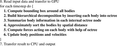 |
| Figure 6.1
Pseudo code of the Barnes Hut algorithm; bold print denotes GPU code.
|
Figure 6.2
Figure 6.3
Figure 6.4
and
Figure 6.5
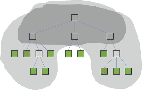
illustrate the operation of kernels 1, 2, 3, and 5. Kernel 1 computes a bounding box around all bodies; this box becomes the root node of the octree (i.e., the outermost cell). Kernel 2 hierarchically subdivides this cell until there is at most one body per innermost cell. This is accomplished by inserting all bodies into the octree. Kernel 3 computes, for each cell, the center of gravity and the cumulative mass of all contained bodies (Figure 6.4
shows this for the two shaded
cells). Kernel 4 (no figure) sorts the bodies according to an in-order traversal of the octree, which typically places spatially close bodies close together. Kernel 5 computes the forces acting on each body. Starting from the octree's root, it checks whether the center of gravity is far enough away from the current body for each encountered cell (the current body is located at the source of the arrows in
Figure 6.5
). If it is not (solid arrow), the subcells are visited to perform a more accurate force calculation (the three dotted arrows); if it is (single dashed arrow), only one force calculation with the cell's center of gravity and mass is performed, and the subcells and all bodies within them are not visited, thus greatly reducing the total number of force calculations. Kernel 6 (no figure) nudges all the bodies into their new positions and updates their velocities.
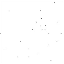 |
| Figure 6.2
Bounding box kernel (kernel 1).
|
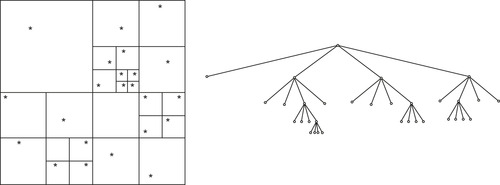 |
| Figure 6.3
Hierarchical decomposition kernel (kernel 2); 2-D view on left, tree view on right.
|
 |
| Figure 6.4
Center-of-gravity kernel (kernel 3).
|
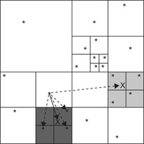 |
| Figure 6.5
Force calculation kernel (kernel 5).
|
This section describes our CUDA implementation of the Barnes Hut algorithm, with a focus on the optimizations we incorporated to make it execute efficiently on a GPU. We start with the global optimizations that apply to all kernels and then discuss each kernel individually. The section concludes with a summary and general optimization patterns that may be useful for speeding up other irregular codes.
6.3.1. Global Optimizations
Dynamic data structures such as trees are typically built from heap objects, where each heap object contains multiple fields, e.g., child-pointer and data fields, and is allocated dynamically. Because dynamic allocation of and accesses to heap objects tend to be slow, we use an array-based data structure. Accesses to arrays cannot be coalesced if the array elements are objects with multiple fields, so we use several aligned scalar arrays, one per field, as outlined in
Figure 6.6
. As a consequence, our code uses array indexes instead of pointers to tree nodes.
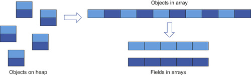 |
| Figure 6.6
Using multiple arrays (one per field) instead of an array of objects or separate heap objects.
|
In Barnes Hut, the cells, which are the internal tree nodes, and the bodies, which are the leaves of the tree, have some common fields (e.g., the mass and the position). Other fields are only needed by either the cells (e.g., the child pointers) or the bodies (e.g., the velocity and the acceleration). However, to simplify and speed up the code, it is important to use the same arrays for both bodies and cells.
We allocate the bodies at the beginning and the cells at the end of the arrays, as illustrated in
Figure 6.7
and use an index of
 as a “null pointer.” This allocation order has several advantages. First, a simple comparison of the array index with the number of bodies determines whether the index points to a cell or a body. Second, in some code sections, we need to find out whether an index refers to a body or to null. Because
 is also smaller than the number of bodies, a single integer comparison suffices to test both conditions. Third, we can alias arrays that hold only cell information with arrays that hold only body information to reduce the memory consumption while maintaining a one-to-one correspondence between the indexes into the different arrays, thus simplifying the code.
Figure 6.7
shows how arrays A and B are combined into array AB.
is also smaller than the number of bodies, a single integer comparison suffices to test both conditions. Third, we can alias arrays that hold only cell information with arrays that hold only body information to reduce the memory consumption while maintaining a one-to-one correspondence between the indexes into the different arrays, thus simplifying the code.
Figure 6.7
shows how arrays A and B are combined into array AB.
 |
| Figure 6.7
Array layout and element allocation order for body-only (A), cell-only (B), and combined (AB) arrays;
|
Our implementation requires compute capability 1.2, in particular, a thread-voting function as well as the larger number of registers, which allows launching more threads per block. The thread count per block is maximized and rounded down to the nearest multiple of the warp size for each kernel. All kernels use at least as many blocks as there are streaming multiprocessors in the GPU, which is automatically detected.
Because all parameters passed to the kernels, such as the starting addresses of the various arrays, stay the same throughout the time step loop, we copy them once into the GPU's constant memory. This is much faster than passing them with every kernel invocation.
Our code does not transfer any data between the CPU and the GPU except for one initial transfer to send the input to the GPU and one final transfer to send the result back to the CPU. This approach avoids slow data transfers over the PCI bus during the simulation and is possible because we execute the entire algorithm on one GPU.
Because our code operates on octrees in which nodes can have up to eight children, it contains many loops with a trip count of eight. We use pragmas to unroll these loops, though the compiler does this by default in most cases.
6.3.2. Kernel 1 Optimizations
The first kernel computes a bounding box around all bodies, i.e., the root of the octree. To do that, it has to find the minimum and maximum coordinates in the three spatial dimensions. First, the kernel breaks
up the data into equal sized chunks and assigns one chunk to each block. Each block then performs a reduction operation that follows the example outlined in Section B.5 of the CUDA Programming Guide
[5]
. All the relevant data in main memory are read only once and in a fully coalesced manner. The reduction is performed in shared memory in a way that avoids bank conflicts and minimizes thread divergence
[6]
. The only thread divergence occurs at the very end when there are fewer than 32 elements left to process per block. Our implementation uses the built-in
min
and
max
functions to perform the reduction operations, since these are faster than
if
statements. The final result from each block is written to main memory. The last block, as is determined by a global
atomicInc
operation, combines these results and generates the root node.
6.3.3. Kernel 2 Optimizations
The second kernel implements an iterative tree-building algorithm that uses lightweight locks, only locks child pointers of leaf cells, and deliberately slows down unsuccessful threads to reduce the memory pressure. The bodies are assigned to the blocks and threads within a block in round-robin fashion. Each thread inserts its bodies one after the other by traversing the tree from the root to the desired last-level cell and then attempts to lock the appropriate child pointer (an array index) by writing an otherwise unused value ( ) to it using an atomic operation, as illustrated in
Figures 6.8
and
6.9
. If the locking succeeds, the thread inserts the new body, thereby overwriting the lock value, which releases the lock. If a body is already stored at this location, the thread first creates a new cell by atomically requesting the next unused array index, inserts the original and the new body into this new cell, executes a memory fence (__threadfence
) to ensure the new subtree is visible to the rest of the cores, and then attaches the new cell to the tree, thereby releasing the lock.
) to it using an atomic operation, as illustrated in
Figures 6.8
and
6.9
. If the locking succeeds, the thread inserts the new body, thereby overwriting the lock value, which releases the lock. If a body is already stored at this location, the thread first creates a new cell by atomically requesting the next unused array index, inserts the original and the new body into this new cell, executes a memory fence (__threadfence
) to ensure the new subtree is visible to the rest of the cores, and then attaches the new cell to the tree, thereby releasing the lock.
 |
| Figure 6.8
Locking the dashed child “pointer” of the starred cell to insert a body.
|
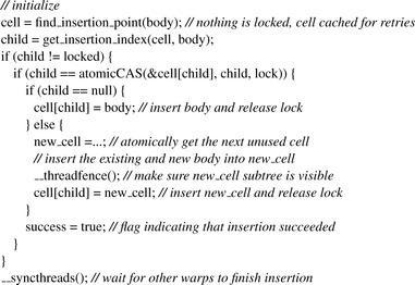 |
| Figure 6.9
Pseudo code for inserting a body.
|
The threads that fail to acquire a lock have to retry until they succeed. Allowing them to do so right away would swamp the main memory with requests and slow down the progress of the successful threads, especially in the beginning when the tree is small. As long as at least one thread per warp (a warp is a group of threads that execute together) succeeds in acquiring a lock, thread divergence temporarily disables all the threads in the warp that did not manage to acquire a lock until the successful threads have completed their insertions and released their locks. This process greatly reduces
the number of retries (i.e., memory accesses), most of which would be useless because they would find the lock to still be unavailable. To also prevent warps in which
all
threads fail to acquire a lock from flooding the memory with lock-polling requests, we inserted an artificial barrier (__syncthreads
) into this kernel (the last line in the pseudo code in
Figure 6.9
) that is not necessary for correctness. This barrier throttles warps that would otherwise most likely not be able to make progress but would slow down the memory accesses of the successful threads. The code shown in
Figure 6.9
executes inside of a loop that moves on to the next body assigned to a thread whenever the success flag is true.
In summary, this kernel employs the following optimizations. It caches the root's data in the register file. It employs a barrier to throttle threads that fail to acquire a lock. It minimizes the number of locks by only locking child pointers of leaf cells. It employs lightweight locks that require a single atomic operation to lock and a memory fence followed by a store operation to release the lock. The common case, that is, adding a body without the need to generate a new cell (typically, about one cell is created per three bodies), uses an even faster unlock mechanism that requires only a store operation, but no memory fence.
6.3.4. Kernel 3 Optimizations
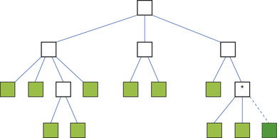
The third kernel traverses the unbalanced octree from the bottom up to compute the center of gravity and the sum of the masses of each cell's children.
Figure 6.10
shows the octree nodes in the global arrays (bottom) and the corresponding tree representation (top). In this kernel, the cells are assigned to the blocks and to the threads within a block in round-robin fashion. Note that the leftmost cell is not necessarily mapped to the first thread in the first block. Rather, it is mapped to the thread that yields the correct alignment to enable coalescing of memory accesses.
 |
| Figure 6.10
Allocation of bodies (the shaded nodes) and cells (the white nodes) in the global arrays and corresponding tree representation; the numbers represent thread IDs.
|
Initially, all cells have negative masses, indicating that their true masses still need to be computed. Because the majority of the cells in the octree have only bodies as children, the corresponding threads
can immediately compute the cell data. In fact, this can be done using coalesced accesses to store the mass and position information until the threads in a warp start processing cells whose children are not yet ready — this step forces threads to wait different amounts of time.
Because the allocation order ensures that a cell's children have lower array indexes than the cell does, it is not possible that a thread will ever attempt to process a cell before it has processed all tree successors of this cell that are assigned to this thread. For example, threads 3 and 4 both have two cells on the same path assigned to them in
Figure 6.10
, but they are guaranteed to first process the lower-level cell. If this were not the case, the code could deadlock.
As the pseudo code in
Figure 6.11
shows, the computed center of gravity is stored first, then a memory fence is executed, and finally the computed mass is stored to indicate that the cell's data are now ready. The memory fence ensures that no other thread in the GPU can see the updated mass before it sees the updated center of gravity. This way, no locks or atomic operations are necessary, and preexisting memory locations (the mass fields) serve as ready flags. Unsuccessful threads have to poll until the “ready flag” is set. Note that the code shown in
Figure 6.11
executes inside of a loop that moves on to the next cell assigned to the thread whenever the success flag is set to true.
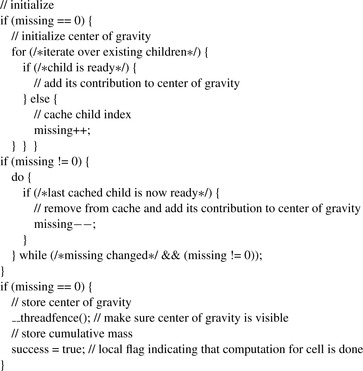 |
| Figure 6.11
Pseudo code for computing a cell's center of gravity.
|
For performance reasons, the kernel caches all the child pointers of the current cell in shared memory that point to not-ready children. This way, the thread polls only the missing children, which reduces main memory accesses. Moreover, if a child is found to still be unready, thread divergence (due to exiting the do-while loop in
Figure 6.11
) deliberately forces the thread to wait for a while before trying again to throttle polling requests.
Kernel 3 performs two more functions (not included in
Figure 6.11
) that piggyback on its bottom-up traversal and therefore incur little additional runtime. The first extra operation is to count the bodies in all subtrees and store this information in the cells. These counts make kernel 4 much faster. The second additional operation is to move all non-null child pointers to the front. In the earlier kernels, the
position of each child is essential for correct operation, but the later kernels just need to be able to visit all children. Hence, we can move the existing children to the front of the eight-element child array in each cell and move all the nulls to the end. This makes kernel 5 faster.
In summary, this kernel includes the following optimizations: It maps cells to threads in a way that results in good load balance, avoids deadlocks, allows some coalescing, and enables bottom-up traversals without explicit parent pointers. It does not require any locks or atomic operations, uses a data field in the cells as a ready flag, and sets the flags with a memory fence followed by a simple write operation. It throttles unsuccessful threads, caches data, and polls only missing data to minimize the number of main memory accesses. Finally, it moves the children in each cell to the front and records the number of bodies in all subtrees to accelerate later kernels.
6.3.5. Kernel 4 Optimizations
This kernel sorts the bodies in parallel using a top-down traversal. It employs the same array-based traversal technique as the previous kernel except that the processing order is reversed; i.e., each thread starts with the highest array index assigned to it and works its way down. It also uses a data field as a ready flag. Based on the number of bodies in each subtree, which was computed in kernel 3, it concurrently places the bodies into an array such that the bodies appear in the same order in the array as they would during an in-order traversal of the octree. This sorting groups spatially close bodies together, and these grouped bodies are crucial to speed up kernel 5.
The fifth kernel requires the vast majority of the runtime and is therefore the most important to optimize. It assigns all bodies to the blocks and threads within a block in round-robin fashion. For each body, the corresponding thread traverses some prefix of the octree to compute the force acting upon this body, as illustrated in
Figure 6.12
. These prefixes are similar for spatially close bodies, but different for spatially distant bodies. Because threads belonging to the same warp execute in lockstep, every warp in this kernel effectively has to traverse the union of the tree prefixes of all the threads in the warp. In other words, whenever a warp traverses a part of the tree that some of the threads do not need, those threads are disabled due to thread divergence, but they still have to wait for this part to be traversed. As a consequence, it is paramount to group spatially nearby bodies together so that the threads in a warp have to traverse similar tree prefixes, that is, to make the union of the prefixes as small as possible. This is why the sorting in kernel 4 is so important. It eliminates most of the thread divergence and accelerates kernel 5 by an order of magnitude. In fact, we opted to eliminate this kind of thread divergence entirely because it is pointless to make some threads wait when they can, without incurring additional runtime, improve the accuracy of their computation by expanding their tree prefix to encompass the entire union. Determining the union's border can be done extremely quickly using the
__all
thread-voting function, as illustrated in
Figure 6.13
.
 |
| Figure 6.12
Tree prefixes that need to be visited for the two marked bodies.
|
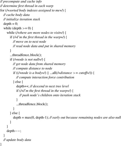 |
| Figure 6.13
Pseudo code of the force calculation kernel.
|
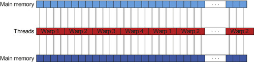
Having eliminated thread divergence and reduced the amount of work each warp has to do by minimizing the size of the union of the prefixes, we note that main memory accesses still pose a major performance hurdle because this kernel contains very little computation with which to hide them. Moreover, the threads in a warp always access the same tree node at the same time; that is, they always read from the same location in main memory. Unfortunately, multiple reads of the same address are not coalesced by older GPU hardware, but instead result in multiple separate accesses. To remedy this situation, we allow only one thread per warp to read the pertinent data, and then that thread makes the data
available to the other threads in the same warp by caching the data in shared memory. This introduces brief periods of thread divergence but reduces the number of main memory accesses by a factor of 32, resulting in a substantial speedup of this memory-bound kernel. The code needs a block-local memory fence (__threadfence_block()
) to prevent data reordering so that the threads in a warp can safely retrieve the data from shared memory. Note that the shared memory allows all threads to simultaneously read the same location without bank conflict.
In addition to these two major optimizations (i.e., minimizing the amount of work per warp and minimizing the number of main memory accesses), kernel 5 incorporates the following optimizations, some of which are illustrated in
Figure 6.13
. It does not write to the octree and therefore requires no locks or ready flags. It caches information that depends only on the tree-depth of a node in shared memory, it uses the built-in
rsqrtf
function to quickly compute “one over square root,” it uses only
one thread per warp to control the iteration stack (which is necessary to avoid recursion) to reduce the memory footprint enough to make it fit into shared memory, and it takes advantage of the children having been moved to the front in kernel 3 by stopping the processing of a cell's children as soon as the first null entry is encountered. This early termination reduces thread divergence because it makes it likely that all threads in a warp find their first few children to be non-null and their last few children to be null. This is another example of grouping similar work together to minimize divergence and maximize performance.
6.3.7. Kernel 6 Optimizations
The sixth kernel updates the velocity and position of each body based on the computed force. It is a straightforward, fully coalesced, nondivergent streaming kernel, as illustrated in
Figure 6.14
. As in the other kernels, the bodies are assigned to the blocks and threads within a block in round-robin fashion.
 |
| Figure 6.14
Fully coalesced streaming updates of the body positions and velocities.
|
6.3.8. Optimization Summary
This subsection summarizes the optimizations described above and highlights general principles we believe may be useful for tuning CUDA implementations of other irregular pointer-chasing codes.
Table 6.1
combines the optimizations from the various Barnes Hut kernels and groups them by category.
In implementing the Barnes Hut algorithm in CUDA and tuning it, we found the following general optimization principles to be important.
Maximizing Parallelism and Load Balance
To hide latencies, particularly memory latencies, it is important to run a large number of threads and blocks in parallel. By parallelizing every step of our algorithm across threads and blocks as well as by using array elements instead of heap objects to represent tree nodes, we were able to assign balanced amounts of work to any number of threads and blocks.
Minimizing Thread Divergence
To maintain maximum parallelism, it is important for the threads in a warp to follow the same control flow. We found that grouping similar work together can drastically reduce thread divergence, especially in irregular code.
Minimizing Main Memory Accesses
Probably the most important optimization for memory-bound code is to reduce main memory accesses as much as possible, for example, by caching data and by throttling warps that are likely to issue memory accesses that do not contribute to the overall progress.
By grouping similar work together in the same warp, we managed to greatly increase sharing and thus reduce main memory accesses. By throttling warps in which all threads failed to acquire a lock and by allowing threads to poll only as-yet unready data, we were able to further reduce the amount of main memory traffic.
Using Lightweight Locks
If locking is necessary, as few items as possible should be locked and for as short a time as possible. For example, we never lock nodes, only last-level child pointers. The locking is done with an atomic operation, and the unlocking is done with an even faster memory fence and store operation. For maximum speed and minimum space overhead, we use existing data fields instead of separate locks and utilize otherwise unused values to lock them. Writing to these fields releases the lock. In some cases, no atomic operations are needed at all because a fence and store operation suffices to achieve the necessary functionality.
Combining Operations
Because pointer-chasing operations are particularly expensive on GPUs, it is probably worthwhile to combine tasks to avoid additional traversals. For example, our code computes the mass and center of gravity, counts the bodies in the subtrees, and moves the non-null children to the front in a single traversal.
Maximizing Coalescing
Coalesced memory accesses are difficult to achieve in irregular pointer-chasing codes. Nevertheless, by carefully allocating the node data and spreading the fields over multiple scalar arrays, we have managed to attain some coalescing in several kernels.
Avoiding GPU/CPU Transfers
Copying data to or from the GPU is a relatively slow operation. However, data can be left on the GPU between kernels. By implementing the entire algorithm on the GPU, we were able to eliminate almost all data transfers between the host and the device. Moreover, we used the constant memory to transfer kernel parameters — a process that is significantly faster and avoids retransmitting unchanged values.
6.4. Evaluation and Validation of Results, Total Benefits, and Limitations
6.4.1. Evaluation Methodology
Implementations
In addition to our parallel CUDA version of the Barnes Hut algorithm, we wrote two more implementations for comparison purposes: (1) a serial C version of the Barnes Hut algorithm and
(2) a parallel CUDA version of the
 algorithm. The three implementations use single precision. The
 algorithm computes all pair-wise forces and is therefore more precise than the approximate Barnes Hut algorithm. The Barnes Hut implementations are run with a tolerance factor of 0.5. The C and CUDA versions include many of the same optimizations, but also CPU and GPU specific optimizations, respectively.
Inputs
We generated five inputs with 5000, 50,000, 500,000, 5,000,000, and 50,000,000 galaxies (bodies). The galaxies’ positions and velocities are initialized according to the empirical Plummer model
[2]
, which mimics the density distribution of globular clusters.
System
We evaluated the performance of our CUDA implementation on a 1.3 GHz Quadro FX 5800 GPU with 30 streaming multiprocessors (240 cores) and 4 GB of main memory. For performance comparison purposes and as host device, we used a 2.53 GHz Xeon E5540 CPU with 48 GB of main memory.
Compilers
We compiled the CUDA codes with
nvcc
v3.0 and the “-O3 -arch=sm_13” flags. For the C code, we used
icc
v11.1 and the “-O2” flag because it generates a faster executable than
nvcc
's underlying C compiler does.
Metric
We reported the best runtime of three identical experiments. There is typically little difference between the best and the worst runtimes. We measured only the time step loop; that is, generating the input and writing the output is not included in the reported runtimes.
Validation
We compared the output of the three codes to verify that they are computing the same result. Note, however, that the outputs are not entirely identical because the
 algorithm is more accurate than the Barnes Hut algorithm and because the CPU's floating-point arithmetic is more precise than the GPU's.
6.4.2. Results
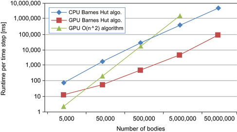
Figure 6.15
plots the runtime per time step versus the problem size on a log-log scale for the three implementations (lower numbers are better). With increasing input size, the parallel CUDA Barnes Hut code is 5, 35, 66, 74, and 53 times faster than the serial C code. So even on this irregular code, the GPU has an over 50x performance advantage over a single CPU core for large enough problem sizes. The benefit is lower with small inputs primarily because the amount of parallelism is lower. Our kernels launch between 7680 and 23,040 threads, meaning that many threads receive no work with our smallest input. We are not sure why the performance advantage with the largest input is lower than with the second-largest input. It takes the GPU just over 5 seconds per time step to simulate 5,000,000 bodies and 88 seconds for 50,000,000 bodies.
 |
| Figure 6.15
Runtime per simulated time step in milliseconds.
|
For problem sizes below about 10,000 bodies, the
 CUDA implementation is the fastest. On the evaluated input sizes, the Barnes Hut CUDA code is 0.2, 3.3, 35, and 314 times faster than the
 CUDA code. We did not run the largest problem size with the
 algorithm as it would have taken almost two days to complete one time step. Because the Barnes Hut algorithm requires only
 operations, its benefit over the
 algorithm increases rapidly with larger problem sizes.
Table 6.2
lists the running times of each kernel and compares them with the corresponding running times on the CPU. The CPU/GPU ratio roughly approximates the number of CPU cores needed to match the GPU performance. Kernel 5 (force calculation) is by far the slowest, followed by kernel 2
(tree building). The remaining four kernels represent less than 3% of the total running time on the GPU and 0.5% on the CPU. The GPU is faster than a single CPU core on each kernel by a substantial margin. Kernels 2, 3, and 4 are under 10 times faster, whereas the remaining kernels are over 60 times faster. The most important kernel, kernel 5, is over 90 times faster. These results indicate that a hybrid approach, where some of the work is performed on the CPU, is unlikely to result in much benefit, even if the CPU code is parallelized across multiple cores and there is no penalty for transferring data between the CPU and the GPU.
Table 6.3
compares the two CUDA versions in terms of their runtime, floating-point operations per second, and bytes accessed in main memory per second for an input of 5,000,000 bodies. The results are for all kernels combined and show that the very regular
 code utilizes the GPU hardware at almost maximum effectively, whereas the irregular Barnes Hut code does not. Nevertheless, the Barnes Hut implementation reaches a respectable 75 Gflop/s. Its main memory throughput is low in part because of uncoalesced accesses and in part because we allow only one of the 32 threads in a warp to access main memory on behalf of all threads. The remaining threads operate almost exclusively on data in shared memory.
Other than
 CUDA implementations
[3]
, there are no implementations of an entire
CUDA implementations
[3]
, there are no implementations of an entire
 -body algorithm on the GPU that we are aware of. Our approach of running the entire Barnes Hut algorithm on the GPU avoids slow data transfers between the CPU and the GPU, but it also limits the maximum problem size to just over 50,000,000 bodies on our hardware. Other approaches that execute part of the work on the CPU may be more suitable for larger problem sizes. For example, a recent implementation by Hamada
et al.
[4]
uses the CPU to construct the tree, traverse the tree, perform the time integration, and send interaction lists to the GPU. The GPU then computes the forces between the bodies in the interaction lists in a streaming fashion that is not limited by the amount of memory on the GPU.
-body algorithm on the GPU that we are aware of. Our approach of running the entire Barnes Hut algorithm on the GPU avoids slow data transfers between the CPU and the GPU, but it also limits the maximum problem size to just over 50,000,000 bodies on our hardware. Other approaches that execute part of the work on the CPU may be more suitable for larger problem sizes. For example, a recent implementation by Hamada
et al.
[4]
uses the CPU to construct the tree, traverse the tree, perform the time integration, and send interaction lists to the GPU. The GPU then computes the forces between the bodies in the interaction lists in a streaming fashion that is not limited by the amount of memory on the GPU.
Our implementation is based on the classical Barnes Hut algorithm
[1]
instead of the newer method by Barnes
[7]
. The classical method allows only one body per leaf node in the tree, whereas the newer approach allows multiple bodies per node and therefore requires a substantially smaller tree. As a result, the traversal time is much reduced, making the new algorithm a better candidate for a GPU implementation
[4]
. We opted to use the classical algorithm because we are interested in finding general ways to make tree codes efficient on GPUs as opposed to focusing exclusively on the Barnes Hut algorithm.
6.4.4. Conclusions
The main conclusion of our work is that GPUs can be used to accelerate irregular codes, not just regular codes. However, a great deal of programming effort is required to achieve good performance. We estimate that it took us two person months to port our preexisting C implementation to CUDA and optimize it. In particular, we had to completely redesign the main data structure, convert all the recursive code into iterative code, explicitly manage the cache (shared memory), and parallelize the implementation both within and across thread blocks. The biggest performance win, though, came from turning some of the unique architectural features of GPUs, which are often regarded as performance hurdles for irregular codes, into assets. For example, because the threads in a warp necessarily run in lockstep, we can have one thread fetch data from main memory and share them with the other threads without the need for synchronization. Similarly, because barriers are implemented in hardware on GPUs and are extremely fast, we have been able to use them to reduce wasted work and main memory accesses in a way and to an extent that is impossible in current CPUs because barrier implementations in CPUs have to communicate through memory.
We are actively working on writing high-performing CUDA implementations for other irregular algorithms. The goal of this work is to identify common structures and optimization techniques that can be generalized so that they are ultimately useful for speeding up entire classes of irregular programs.
Acknowledgments
This work was supported in part by NSF grants CSR-0923907, CSR-0833162, CSR-0752845, CSR-0719966, and CSR-0702353 as well as gifts from IBM, Intel, and NEC. The results reported in this chapter have been obtained on resources provided by the Texas Advanced Computing Center (TACC) at the University of Texas at Austin.
References
[1]
J. Barnes, P. Hut,
A hierarchical O(n
log
n
) force-calculation algorithm
,
Nature
324
(4
) (1986
)
446
–
449
.
[2]
H.C. Plummer,
On the problem of distribution in globular star clusters
,
Mon. Not. R. Astron. Soc.
71
(1911
)
460
–
470
.
[3]
L. Nyland, M. Harris, J. Prins,
Fast n-body simulation with CUDA
,
In: (Editor: H. Nguyen)
GPU Gems
,
3
(2007
)
Addison-Wesley Professional
;
(Chapter 31)
.
[4]
T. Hamada, K. Nitadori, K. Benkrid, Y. Ohno, G. Morimoto, T. Masada, et al., A novel multiple-walk parallel algorithm for the Barnes-Hut treecode on GPUs — towards cost effective, high performance N-body simulation, vol. 24 (1–2), SpringerLink, Computer Science — Research and Development, Springer-Verlag, New York, 2009 (special issue paper).
[5]
NVIDIA
,
CUDA Programming Guide, Version 2.2
. (2009
)
NVIDIA Corp.
,
Santa Clara, CA
.
[6]
D. Kirk, W.W. Hwu, Lecture 10,
http://courses.ece.illinois.edu/ece498/al/lectures/lecture10-control-flow-spring-2010.ppt
(accessed 06.11.10).
[7]
J. Barnes,
A modified tree code: don't laugh; it runs
,
J. Comput. Phys.
87
(1
) (1990
)
161
–
170
.
..................Content has been hidden....................
You can't read the all page of ebook, please click here login for view all page.