
Chapter 10. Wavelet-Based Density Functional Theory Calculation on Massively Parallel Hybrid Architectures
Luigi Genovese, Matthieu Ospici, Brice Videau, Thierry Deutsch and Jean-François Méhaut
Electronic structure calculations has become in recent years a widespread tool to predict and investigate electronic properties of physics at the nanoscale. Among the different approaches, the Kohn-Sham (KS) formalism
[1]
in the density functional theory (DFT) framework has certainly become one of the most used. At the same time, the need to simulate systems more and more complex together with the increase in computational power of modern machines pushes the formalism toward limits that were unconceivable just a few years ago. It is thus important to provide reliable solutions to benefit from the enhancements of computational power in order to use these tools in more challenging systems. With this work, we have tried to provide an answer on this direction by exploiting the GPU acceleration of systematic DFT codes. The principal operations of an electronic structure code based on Daubechies wavelets were ported on NVIDIA GPU cards. The CPU version of the code on which our work is based has systematic convergence properties, very high performances, and an excellent efficiency on parallel and massively parallel environments. This code is delivered under the GNU-GPL license and was conceived from the beginning for parallel and massively parallel architectures. For this reason, the questions related to the integration of GPU accelerators into a parallel environment are also addressed. The topics that are presented in this chapter are thus related to efficiently benefiting from GPU acceleration in the context of a complex code made with sections with different runtime behavior. For these reasons, in addition to the technical implementation details of the GPU kernels, a considerable part of the discussion is related to the insertion of these kernels in the context of the full code. The study of GPU accelerations strategies for such a code can be of great interest for a number of groups working on codes with rich and complicated structures.
10.1. Introduction, Problem Statement, and Context
In this contribution, we present an implementation of a full DFT code that can run on massively parallel hybrid CPU-GPU clusters. Our implementation is based on the architecture of NVIDIA GPU cards of compute capability at least of type 1.3, which support double-precision floating-point numbers. This DFT code, named BigDFT, is delivered within the GNU-GPL license either in a stand-alone version or integrated in the ABINIT software package. The formalism of this code is based on Daubechies wavelets
[10]
. As we will see in the following sections, the properties of this basis set are well suited for an extension on a GPU-accelerated environment. In addition to focusing on the implementation
details of a single operation, this chapter also relies of the usage of the GPU resources in a complex code with different kinds of operations.
We start with a brief overview of the BigDFT code in order to describe why and how the use of GPU can be useful for accelerating the code operations.
10.1.1. Overview of the BigDFT Code
In the KS formulation of DFT, the KS wavefunctions
 are eigenfunctions of the KS Hamiltonian operator. The KS Hamiltonian can then be written as the action of three operators on the wavefunction:
 where
where
 is a real-space-based (local) potential. The KS potential
 is a functional of the electronic density of the system:
 where
where
 is the occupation number of orbital
 .
.
(10.1)
(10.2)
The KS potential
 contains the Hartree potential
 , solution of the Poisson's equation
 , the exchange-correlation potential
 , and the external ionic potential
 acting on the electrons. In BigDFT code a pseudopotential term is added to the Hamiltonian matrix, that has a local and a nonlocal term,
 .
.
As usual, in a KS DFT calculation, the application of the Hamiltonian matrix is a part of a self-consistent cycle, needed for minimizing the total energy. In addition to the usual orthogonalization routine, in which scalar products
 should be calculated, another operation that is performed on wavefunctions in BigDFT code is the preconditioning. This is calculated by solving the Helmholtz equation
 where
where
 is the gradient of the total energy with respect to the wavefunction
 , of energy
 . The solution
 is found by solving
Eq. 10.3
by a preconditioned conjugate gradient method.
is found by solving
Eq. 10.3
by a preconditioned conjugate gradient method.
(10.3)
10.1.2. Daubechies Basis and Convolutions
The set of basis functions used to express the KS orbitals is of key importance for the nature of the computational operations that have to be performed. In the BigDFT code, the KS wavefunctions are expressed on Daubechies wavelets. The latter is a set of localized, real-space-based orthogonal functions that allow for a systematic, multiresolution description. These basis functions are centered on the grid points of a mesh that is placed around the atoms, see
Figure 10.1
.
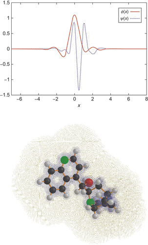 |
| Figure 10.1
An example of a simulation domain for a small molecule analyzed with BigDFT code. Both the atoms and the adaptive mesh that is associated to the basis function are indicated. In the top panel the one-dimensional versions of the Daubechies functions that are associated to a given grid point are plotted.
|
We will see in the following section that, thanks to the properties of the basis functions, the action of the KS operators can be written as three-dimensional convolutions with short, separable filters. A more complete description of these operations can be found in the BigDFT reference paper
[9]
.
To illustrate the action of the local Hamiltonian operator (laplacian plus local potential), we have to represent a given KS wavefunction
 in the so-called fine-scaling function representation, in which the wavefunctions are associated to three-dimensional arrays that express their components. These arrays
contain the components
in the so-called fine-scaling function representation, in which the wavefunctions are associated to three-dimensional arrays that express their components. These arrays
contain the components
 of
of
 in the basis of Daubechies scaling functions
 :
:
(10.4)
10.2.1. The Kinetic Operator
The matrix elements of the kinetic energy operator among the basis functions can be calculated analytically
[9]
and
[16]
. For the pure fine-scaling function representation described in
Eq. 10.4
, the result of the application of the kinetic energy operator on this wavefunction has the expansion coefficients
 , which are related to the original coefficients
 by a convolution
 where
where
 and
and
 are the filters of the one-dimensional second derivative in Daubechies scaling functions basis, which can be computed analytically.
(10.5)
(10.6)
10.2.2. Application of the Local Potential, Magic Filters
The application of the local potential in Daubechies basis consists of the basis decomposition of the function product
 . As explained in
[9]
and
[17]
, the simple evaluation of this product in terms of the point values of the basis functions is not precise enough. A better result may be achieved by performing a transformation to the wavefunction coefficients — this process allows for calculation of the values of the wavefunctions on the fine grid, via a smoothed version of the basis functions. This is the so-called magic filter transformation, which can be expressed as follows:
. As explained in
[9]
and
[17]
, the simple evaluation of this product in terms of the point values of the basis functions is not precise enough. A better result may be achieved by performing a transformation to the wavefunction coefficients — this process allows for calculation of the values of the wavefunctions on the fine grid, via a smoothed version of the basis functions. This is the so-called magic filter transformation, which can be expressed as follows:
 and allows the potential application to be expressed with better accuracy. After application of the local potential (pointwise product), a transposed magic filter transformation can be applied to obtain Daubechies expansion coefficients of
 .
.
(10.7)
10.2.3. The Operations in BigDFT Code
The previously described operations must be combined together for the application of the local Hamiltonian operator
 . The detailed description of how these operations are chained is beyond the scope of this chapter and can be found in the BigDFT reference paper
[9]
. Essentially, the three-dimensional convolutions that correspond to the different operators associated to the local part of the Hamiltonian should be chained one after another.
Figure 10.2
sketches the chain of operations that is performed.
. The detailed description of how these operations are chained is beyond the scope of this chapter and can be found in the BigDFT reference paper
[9]
. Essentially, the three-dimensional convolutions that correspond to the different operators associated to the local part of the Hamiltonian should be chained one after another.
Figure 10.2
sketches the chain of operations that is performed.
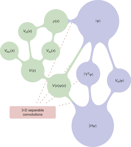 |
| Figure 10.2
A schematic of the application of the Hamiltonian in the BigDFT formalism. The operator
|
The density of the electronic system is derived from the square of the point values of the wavefunctions (see
Eq. 10.2
). As described in
Section 10.1.2
, a convenient way to express the point values of the wavefunctions is to apply the magic filter transformation to the Daubechies basis expansion coefficients.
The local potential
 can be obtained from the local density
 by solving the Poisson's equation and by calculating the exchange-correlation potential
 . These operations are performed via a Poisson Solver based on interpolating scaling functions
[19]
, a basis set tightly connected with Daubechies functions. The properties of this basis are optimal for electrostatic problems, and mixed boundary conditions can be treated explicity. A description of this Poisson solver can be found in papers
[20]
and
[21]
.
. These operations are performed via a Poisson Solver based on interpolating scaling functions
[19]
, a basis set tightly connected with Daubechies functions. The properties of this basis are optimal for electrostatic problems, and mixed boundary conditions can be treated explicity. A description of this Poisson solver can be found in papers
[20]
and
[21]
.
The schematic of all these operations is depicted in
Figure 10.2
.
The application of the Hamiltonian in the BigDFT code is only one of the operations that are performed. During the self-consistent cycle, wavefunctions have to be updated and orthogonalized. Since all the basis functions are orthogonal with each other, the overlap matrices have to be calculated via suitable calls to BLAS routines and then processed with LAPACK subprograms.
An optimized iteration of a KS wavefunction is organized as follows:
1. Local Hamiltonian, construction and application
2. Non-local Hamiltonian
3. Overlap matrix
4. Preconditioning
5. Wavefunction update
6. Orthogonalization (Cholesky factorization)
Steps 1 and 2 have been described in
Figure 10.2
. The application of the non-local Hamiltonian is not treated here and can be found in Ref.
[9]
. The preconditioner (step 4) can also be expressed via a kinetic convolution, as described earlier in this chapter. Steps 3, 5, and 6 are performed via BLAS/LAPACK calls. In the current hybrid implementation, we can execute on the GPU the steps 1 and 4 and also all BLAS routines performed in steps 3 (DGEMM), 5, and 6 (DSYRK, DTRMM). However, all other operations, such as LAPACK routines (step 6) or the multiplication with the nonlocal pseudopotentials (step 2), are still executed on the CPU and can be ported on the GPU. We left these implementations to future versions of the hybrid code.
We have evaluated the amount of time spent for a given operation on a typical run. To do this we have profiled the different sections of the BigDFT code for a parallel calculation. In
Figure 10.8
we show the percent of time that is dedicated to any of the previously described operations, for runs with different architectures. It should be stressed that for the regimes we have tested, there is no hot-spot operation. This makes GPU accelerations more complicated because they will depend on different factors.
10.3. Algorithms, Implementations, and Evaluations
We have seen that the operations that have to be explicitly ported on GPUs is a set of separable three-dimensional convolutions. In the following section, we will show the design and implementation of these operations on NVIDIA GPUs. We start by considering the magic filter application.
10.3.1. From a Separable 3D Convolution to 1D Convolutions
A three-dimensional array
 (input array) of dimension
 (the dimension of the simulation domain of BigDFT) is transformed into the output array
 given by
 With a lowercase index
 we indicate the elements of the input array, while with a capital index
 we indicate the indices after application of the magic filters
 , which have extension from
 to
to
 . The
filter dimension
. The
filter dimension
 equals to the order of the Daubechies family
 , which is 16 in our case. In BigDFT, different boundary conditions (BC) can be applied at the border of the simulation region, which affects the values of the array
s
in (10.8) when the indices are outside bounds.
, which is 16 in our case. In BigDFT, different boundary conditions (BC) can be applied at the border of the simulation region, which affects the values of the array
s
in (10.8) when the indices are outside bounds.
(10.8)
The most convenient way to calculate a three-dimensional convolution of this kind is by combining one-dimensional convolutions and array transpositions, as explained in
[22]
. In fact, the calculation
Eq. 10.8
can be cut in three steps:
1.

 ;
;
2.

 ;
;
3.

 .
.
The final result is thus obtained by a successive application of the same operation:
 The lowest level routine that will be ported on GPU is then a set of
 separate one-dimensional (periodic) convolutions of arrays of size
 , which have to be combined with a transposition. The number
 equals
 ,
,
 and
and
 , respectively, for each step of the three-dimensional construction, while
 ,
,
 , equals the dimension that is going to be transformed. The output of the first step is then taken as the input of the second, and so on.
(10.9)
10.3.2. Kinetic Convolution and Preconditioner
A little, but substantial, difference should be stressed for the kinetic operator application, defined in
Eqs. 10.5
and
10.6
. In this case the three-dimensional filter is the sum of three different filters. This implies that the kinetic filter operation must be cut differently from the other separable convolutions:
1.


2.


3.


Also in this case, the three-dimensional kinetic operator can be seen as a result of a successive application of the same operation:
 In other terms, the one-dimensional kernel of the kinetic energy has two input arrays,
 and
and
 , and returns two output arrays
 and the
 , which is the transposition of
 . At the first step (
 ) we put
 and
and
 . Eventually, for
 , we have
 and
and
 . One can put instead
 , and in that way, will be
 . This algorithm can be also used for the Helmholtz operator of the preconditioner, by putting
 .
.
(10.10)
From the GPU parallelism point of view, there is a set of
 independent convolutions to be computed. Each of the lines of
 elements to be transformed is split in chunks of size
 . Each multiprocessor of the graphic card computes a group of
 different chunks and parallellizes the calculation on its computing units.
Figure 10.3
shows the data distribution on the grid of blocks during the transposition.
different chunks and parallellizes the calculation on its computing units.
Figure 10.3
shows the data distribution on the grid of blocks during the transposition.
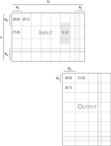 |
| Figure 10.3
Data distribution for 1-D convolution
|
We transfer data from the global to the shared memory of multiprocessors. The shared memory must contain buffers to store the data needed for the convolution computations. In order to perform the convolution for
 elements,
 elements must be sent to the shared memory for the calculation, where
 depends of the size of the convolution filter. The shared memory must thus contain buffers to store the data needed for the convolution computations. The desired boundary condition (for example, periodic wrapping) is implemented in the shared memory during the data transfer. Each thread computes the convolution for a subset of
 elements associated to the block. To avoid bank conflicts, the half-warp size must be a multiple of
 . Each half-warp thus computes at least
 values, and
 is a multiple of that number, chosen in such a way that the total number of elements
 fits in the shared memory. This data distribution is illustrated in
Figure 10.4
.
fits in the shared memory. This data distribution is illustrated in
Figure 10.4
.
 |
| Figure 10.4
Data arrangement in shared memory for a given block. The number of lines
|
10.3.4. Performance Evaluation of GPU Convolution Routines
To evaluate the performance of 1-D convolution routines described in
Eqs. 10.9
and
10.10
, together with the analogous operation for the wavelet transformation, we are going to compare the execution times on a CPU and a GPU. We define the GPU speedup with the ratio between CPU and GPU execution times. For these evaluations, we used a computer with an Intel Xeon Processor X5472 (3 GHz) and a NVIDIA Tesla S1070 card. The CPU version of BigDFT is deeply optimized with optimal loop unrolling and compiler options. The GPU code is compiled with the Intel Fortran Compiler (10.1.011) and the most aggressive compiler options (-O2 -xT
). With these options the magic filter convolutions run at about 3.4 GFlops. All benchmarks are performed with double precision floating-point numbers.
The GPU versions of the one-dimensional convolutions are about one order of magnitude faster than their CPU counterparts. We can then achieve an effective performance rate of the GPU convolutions of about 40 GFlops, by also considering the data transfers in the card. We are not close to peak performance because, on GPU, a considerable fraction of time is still spent in data transfers rather than in calculations. This appears since data should be transposed between input and output array, and the arithmetic needed to perform convolutions is not heavy enough to hide the latency of all the memory transfers. However, we will later show that these results are really satisfying for our purposes.
The performance graphs for the three aforementioned convolutions, together with the compression-decompression operator, are indicated in
Figure 10.5
as a function of the size of the corresponding three-dimensional array.
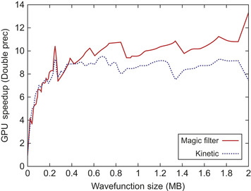 |
| Figure 10.5
Double-precision speedup for the GPU version of the fundamental operations on the wavefunctions as a function of the single wavefunction size.
|
10.3.5. Three-Dimensional Operators, BLAS Routines
As described in the previous sections, to build a three-dimensional operation one must chain three times the corresponding one-dimensional GPU kernels. We obtain in this way the three-dimensional wavelet transformations as well as the kinetic operator and the magic filter transformation (direct and transposed). The multiplication with the potential and the calculation of the square of the wavefunction are performed via the application of some special GPU kernels, based on the same guidelines of the others. The GPU speedup of the local density construction, as well as the local Hamiltonian application and the
preconditioning operation, is represented in
Figure 10.6
as a function of the compressed wavefunction size.
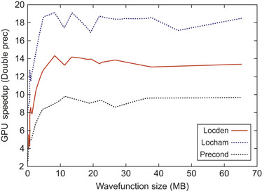 |
| Figure 10.6
Double-precision speedup for the GPU version of the three-dimensional operators used in the BigDFT code as a function of the single wavefunction size.
|
Also the linear algebra operation can be executed on the card thanks to the CUBLAS routines. In
Figure 10.7
we present the speedups we obtain for double-precision calls to CUBLAS routines for a
typical wavefunction size of a BigDFT run as a function of the number of orbitals. These results take into account the amount of time needed to transfer the data of the card.
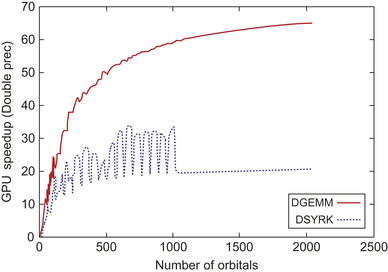 |
| Figure 10.7
Double-precision speedup for the CUBLAS operations used in the code for a typical wavefunction size (300KB) as a function of the number of orbitals.
|
From these tests, we can see that both the GPU-ported sections are an order of magnitude (or more) faster than the corresponding CPU counterpart. We will now consider this behavior in the framework of the complete BigDFT code.
For a code with the complexity of BigDFT, the evaluation of the benefits of using a GPU-accelerated code must be performed at three different levels. First, one has to evaluate the effective speedup provided by the GPU kernels with respect to the corresponding CPU routines that perform the same operations. This is the bare speedup, which, of course, for a given implementation, depends on the computational power that the device can provide us. For the BigDFT code, these results are obtained by analyzing the performances of the GPU kernels that perform the convolutions and the linear algebra (BLAS) operations, as provided by the CUBLAS library. As discussed earlier in this chapter such results can be found in
Figures 10.6
and
10.7
. At the second level, the complete speedup has to be evaluated; the performances of the whole hybrid CPU/GPU code should be analyzed with respect to the pure CPU executions. Clearly, this result depends on the actual importance of the ported routines in the context of the whole code (i.e., following the Amdahl's law). This is the first reliable result of the actual performance enhancements of the GPU porting of the code. For a hybrid code that originates from a monocore CPU program, this is the last level of evaluation. For a parallel code, there is still another step that has to be evaluated. This is the behavior of the hybrid code in a parallel (or massively parallel) environment. Indeed, for parallel runs, the picture is complicated by two things. The first one is the management of the extra level of communication that is introduced by the PCI-express bus, which may interact negatively with the underlying code communication scheduling (MPI or OpenMP par example). The second is the behavior of the code for a number of GPU devices — this number can be lower than the number of CPU processes that are running. In this case the GPU resource is not homogeneously
distributed and the management of this fact adds an extra level of complexity. The evaluation of the code at this stage contributes at the user-level speedup, which is the real time-to-solution speedup.
10.4.1. Parallelization for Homogeneous Computing Clusters (CPU Code)
In its CPU version, two data distribution schemes are used for parallelizing the code. In the orbital distribution scheme (used for Hamiltonian application, preconditioning), each processor works on one or a few orbitals for which it holds all its scaling function and wavelet coefficients. Operations like linear algebra are performed in the coefficient distribution scheme, where each processor holds a certain subset of the coefficients of all the orbitals. The switch between the two different schemes is done via suitable calls to the MPI global transposition routine MPI_ALLTOALLV. This communication scheme, based more on bandwith than latency, guarantees optimal efficiency on parallel and massively parallel architectures.
10.4.2. Performance Evaluation of Hybrid Code
As a test system, we used the ZnO crystal, which has a wurtzite bulk-like structure. Such a system has a relatively high density of valence electrons so that the number of orbitals is rather large even for a moderate number of atoms.
We performed two kinds of tests. For the first one we used the hybrid part of the CINES IBLIS machine, which has 12 nodes, connected with an Infiniband 4X DDR connectX network, each node (2 Xeon X5472 quadri-core) connected with two GPUs on a Tesla S1070 card. To check the behavior of the code for systems of increasing size, we performed a set of calculations for different supercells with an increasing number of processors such that the number of orbitals per MPI processes is kept constant. We performed a comparison for the same runs in which all the CPU cores have a GPU associated. The hybrid code is around 5.5 times faster than its pure CPU couterpart, regardless of the system size.
For the second test we used the hybrid section of the CCRT Titane machine, similar to IBLIS, but with Intel X5570 (Nehalem) CPUs. In this test we kept fixed the size of the system and increased the number of MPI processes in order to decrease the number of orbitals per core. We then controlled the speedup of each run with the hybrid code. The parallel efficiency of the code is not particularly affected by the presence of the GPU. For this machine, owing to the better CPU technology, the time-to-solution speedup is around 3.
Results of the two tests are shown in
Figure 10.8
. Because there is no hot-spot operation, the actual time-to-solution speedup of the complete code is influenced by the features of the code. In other words, a performance evaluation based on the Amdahl's law is of great importance for evaluating the final benefit that a partially accelerated code may have.
These results are interesting and seem very promising for a number of reasons. First of all, as already discussed, not all the routines of the code were ported on the GPU. We focus our efforts to the operators that can be written via a convolution. Also, the application of the nonlocal part of the Hamiltonian (the potential Vnl presented in
Section 10.1.1
) can be performed on the GPU, and we are planning to do this in further developments. Moreover, the actual implementation of the GPU convolutions can be further optimized.
The linear algebra operations also can be further optimized. For the moment, only the calls to the BLAS routines were accelerated on the GPU, via suitable calls to the corresponding CUBLAS routines.
Also the LAPACK routines, which are needed to perform the orthogonalization process, can be ported on a GPU, with a considerable gain. Indeed, the linear algebra operations represent the most expensive part of the code for very large systems
[9]
. An optimization of this section is then crucial for future improvements of the hybrid code.
10.4.3. Parallel Distribution
A typical example of a hybrid architecture may be composed of two quad-core processors and two NVIDIA GPUs. So, in this case, the two GPUs have to be shared among the eight CPU cores. The problem of data distribution and load balancing is a major issue to achieve optimal performance. The operators implemented on the GPU are parallelized within the orbital distribution scheme (see
Section 10.4.1
). This means that each core may host a subset of the orbitals and apply the operators of
Section 10.3.5
only to these wavefunctions.
A possible solution to the GPU sharing is to dedicate statically one GPU to one CPU core. So, in the common configuration, two CPU cores are more powerful because they have access to the GPU. The six other CPU cores do not interact with the GPU. Because the number of orbitals that may be assigned to each core can be adjusted, a possible way to handle the fact that the CPU cores and GPU are in different number would be to assign more orbitals to the cores that have a GPU associated. This kind of approach can be realized owing to the flexibility of the data distribution scheme of BigDFT. However, it may be difficult for the end user to define an optimal repartition of the orbitals between the different cores for a generic system.
For this reason, we have designed an alternative approach where the GPUs are completely shared by all CPU cores. The major consequence is that the set of orbitals is equally distributed to CPU cores. Essentially, each of the CPU cores of a given node is allowed to use one of the GPU cards that are associated to the node so that each card dialogues with a group of CPU cores. Each GPU is associated to two semaphores, which control the memory transfers and the calculations. In this way, the memory transfers of the data between the different cores and the card can be executed asynchronously and overlapped with the calculations. This is optimal because each orbital is processed independently. The schematics of this approach are depicted in
Figure 10.9
.
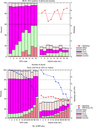 |
| Figure 10.8
Relative speedup of the hybrid DFT code with respect to the equivalent pure CPU run. In the top panel, different runs for systems of increasing size have been done on an Intel X5472 3GHz (Harpertown) machine. In the bottom panel, a given system has been tested with an increasing number of processors on an Intel X5570 2.93GHz (Nehalem) machine. The scaling efficiency of the calculation is also indicated. In the right side of each panel, the same calculation has been done by accelerating the code via one Tesla S1070 card per CPU core used for both architectures. The speedup is around a value of 6 for a Harpertown and around 3.5 for a Nehalem-based calculation.
|
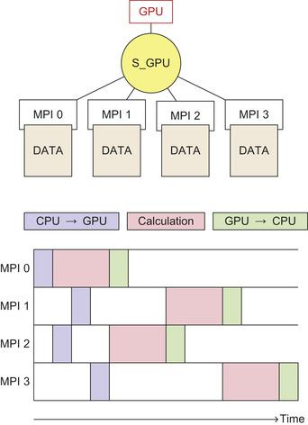 |
| Figure 10.9
Schematic of the management of the association of the same GPU to multiple cores. The time spent on calculation is such that the time needed for data transfer can be hidden by the calculations.
|
For a system of 128 ZnO atoms, we performed different runs for different repartitions of the card per core in order to check the speedup by varying the ratio GPU/CPU on a hybrid run. We then compared this solution with the inhomogeneous data repartition scheme, in which the GPUs are associated statically to two out of eight cores.
Results are plotted in
Table 10.1
. The shared GPU solution provides better performances and speedups than the best possible inhomogeneous data repartition, which is system dependent and much more difficult to tune for the end user. These results are particularly encouraging because at the moment only the convolutions operators are desyncronized by the semaphores (see
Section 10.4.3
), and the
BLAS
routines are executed at the same time on the card. Future improvements in this direction may allow us to better optimize the load on the cards in order to further increase the efficiency.
10.5. Conclusions and Future Directions
The port of the principal sections of an electronic structure code over graphic processing units (GPUs) has been shown. Such GPU sections have been inserted in the complete code in order to have a
production DFT code that is able to run in a multi-GPU environment. The DFT code we used, named BigDFT, is based on Daubechies wavelets, and has high systematic convergence properties, very good performances, and excellent efficiency on parallel computation. The GPU implementation of the code we propose fully respects these properties. We used double-precision calculations, and we might have achieved considerable speedup for the converted routines (up to a factor of 20 for some operations). Our developments are fully compatible with the existing parallellization of the code, and the communication between CPU and GPU does not affect the efficiency of the existing implementation. The data transfers between the CPU and the GPU can be optimized in such a way to allow that more than one CPU core is associated to the same card. This is optimal for modern hybrid supercomputer architectures in which the number of GPU cards is generally smaller than the number of CPU cores. We test our implementation by running systems of variable numbers of atoms on a 12-node hybrid machine, with two GPU cards per node. These developements produce an overall speedup on the whole code of a factor of around six, also for a fully parallel run. It should be stressed that, for these runs, our code has no hot-spot operations, and that all the sections that are ported on the GPU contribute to the overall speedup.
At present, developments in several directions are under way to further increase the efficiency of the usage of the GPU in the context of BigDFT. Different developments are active at present, including the following ones:
• With the advent of the Nehalem processor, we have seen that the CPU power is increased to an extent as to renormalize the cost of the CPU operations that have been GPU ported. The evaluation of the hybrid code with the new generation of Fermi card is thus of great importance to understand the better implementation strategies for the next generation of architectures. Also the combination of GPU acceleration with OMP parallelization (which exists in pure CPU BigDFT code) should be exploited.
• The OpenCL specifications is a great opportunity to build an accelerated code that can be potentially multiplatform. To this aim, an OpenCL version of BigDFT is under finalization, and it has already been tested with new NVIDIA drivers. The development of this version will allow us to implement new functionalities (e.g., different boundary conditions) that have not been implemented in the CUDA version because of lack of time. On the other hand, other implementations of the convolutions routines can be tested, which may fit better with the specifications of the new architectures. In
Figure 10.10
we show some preliminary results in these directions. We have profiled the whole code for different parallelization strategies (OpenMP, MPI), with the addition of GPU acceleration, with CUDA or OpenCL written routines. Two platforms have been used, a Nehalem processor plus an S1070 card, and a Harpertown processor plus a Fermi C2050 card. In both cases, better performances are achieved while combining MPI parallelization with GPU acceleration. In particular, in the Fermi card, we are starting to experience benefits from the concurrent kernel execution. Different strategies are under analysis to show how to efficiently profit from this feature.
• For the same reasons, the strategy of the repartition of the GPU resource also should be reworked. In particular, the possiblity of the concurrent kernel execution should be allowed whenever possible, and the strategies of GPU repartition should be adapted accordingly.
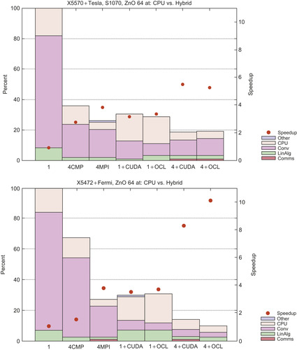 |
| Figure 10.10
Top panel: performances of a run of the BigDFT code for a 64-atom ZnO system on a platform with one Nehalem quad-core and a Tesla S1070 card. The maximum speedup is obtained with combined usage of MPI and CUDA routines, distributed via an S_GPU approach. Bottom panel: the same runs on a platform of one Harpertown and a Fermi C2050. In that case, the concurrent kernel execution, exploited on the OpenCL version of the code, is providing us a benefit, and the speedup grows up to a factor of 10. The study of the exploitation of these strategies for a massively parallel architecture is under way.
|
The hybrid BigDFT code, like its pure CPU counterpart, is available under the GNU-GPL license and can be downloaded from the site shown in reference
[9]
.
[1]
W. Kohn, L.J. Sham,
Phys. Rev.
140
(1965
)
A1133
.
[2]
NVIDIA CUDA Programming Guide, version 3.1, Available from:
http://www.nvidia.com/object/cuda_home.html
.
[3]
J. Yang,
et al.
,
J. Comput. Phys.
221
(2007
)
779
.
[4]
A. Anderson,
et al.
,
Comput. Phys. Commun.
177
(2007
)
298
.
[5]
K. Yasuda,
J. Chem. Theory Comput.
4
(2008
)
1230
.
[6]
K. Yasuda,
J. Comput. Chem.
29
(2008
)
334
–
342
.
[8]
D. Göddeke,
et al.
,
Parall. Comput.
33
(2007
)
10685
.
[9]
L. Genovese,
et al.
,
J. Chem. Phys
129
(2008
)
014109
;
L. Genovese,
et al.
,
J. Chem. Phys.
131
(2009
)
034103
;
Available from:
http://inac.cea.fr/sp2m/L Sim/BigDFT
.
[10]
I. Daubechies,
Ten Lectures on Wavelets
. (1992
)
SIAM
,
Philadelphia, PA
.
[11]
X. Gonze, J.-M. Beuken, R. Caracas, F. Detraux, M. Fuchs, G.-M. Rignanese,
et al.
,
Comput. Mater. Sci.
25
(2002
)
478
–
492
;
Available from:
http://www.abinit.org
.
[12]
S. Goedecker, M. Teter, J. Hutter,
Phys. Rev. B
54
(1996
)
1703
.
[13]
C. Hartwigsen, S. Goedecker, J. Hutter,
Phys. Rev. B
58
(1998
)
3641
.
[14]
M. Krack,
Theor. Chem. Acc.
114
(2005
)
145
.
[15]
S. Goedecker, Wavelets and their Application for the Solution of Partial Differential Equations (ISBN 2-88074-398-2), Presses Polytechniques Universitaires Romandes, Lausanne, Switzerland, 1998.
[16]
G. Beylkin,
SIAM J. Numer. Anal.
6
(1992
)
1716
.
[17]
A.I. Neelov, S. Goedecker,
J. Comput. Phys.
217
(2006
)
312
–
339
.
[18]
J.R. Shewchuk, An Introduction to the Conjugate Gradient Method Without the Agonizing Pain, Unpublished Draft, Carnegie Mellon University, Pittsburgh, PA, Technical Report CS-94-125, (1994). Available from:
http://www.cs.cmu.edu/quake-papers/painless-conjugate-gradient.pdf
.
[19]
G. Deslauriers, S. Dubuc,
Constr. Approx.
5
(1989
)
49
.
[20]
L. Genovese, T. Deutsch, A. Neelov, S. Goedecker, G. Beylkin,
Efficient solution of Poisson's equation with free boundary conditions
,
J. Chem. Phys.
125
(2006
)
074105
.
[21]
L. Genovese, T. Deutsch, S. Goedecker,
Efficient and accurate three-dimensional Poisson solver for surface problems
,
J. Chem. Phys.
127
(2007
)
054704
.
[22]
S. Goedecker,
Rotating a three-dimensional array in optimal positions for vector processing: case study for a three-dimensional fast Fourier transform
,
Comput. Phys. Commun.
76
(1993
)
294
.
[23]
S. Goedecker, A. Hoisie,
Performance Optimization of Numerically Intensive Codes (ISBN 0-89871-484-2)
. (2001
)
SIAM
,
Philadelphia, PA
.
..................Content has been hidden....................
You can't read the all page of ebook, please click here login for view all page.