
Chapter 13. GPU-Supercomputer Acceleration of Pattern Matching
Ali Khajeh-Saeed and J.Blair Perot
This chapter describes the solution of a single very large pattern-matching search using a supercomputing cluster of GPUs. The objective is to compare a query sequence that has a length on the order of
 with a “database” sequence that has a size on the order of roughly
 , and find the locations where the test sequence best matches parts of the database sequence. Finding the optimal matches that can account for gaps and mismatches in the sequences is a problem that is nontrivial to parallelize. This study examines how to achieve efficient parallelism for this problem on a single GPU and between the GPUs when they have a relatively slow interconnect.
13.1. Introduction, Problem Statement, and Context
Pattern matching in the presence of noise and uncertainty is an important computational problem in a variety of fields. It is widely used in computational biology and bioinformatics. In that context DNA or amino acid sequences are typically compared with a genetic database. More recently optimal pattern-matching algorithms have been applied to voice and image analysis, as well as to the data mining of scientific simulations of physical phenomena.
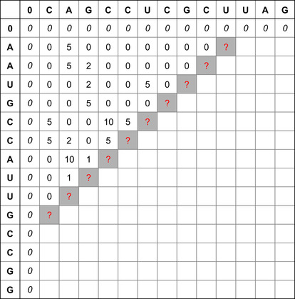
The Smith-Waterman (SW) algorithm is a dynamic programming algorithm for finding the optimal alignment between two sequences once the relative penalty for mismatches and gaps in the sequences is specified. For example, given two RNA sequences, CAGCCUCGCUUAG (the database) and AAUGCCAUUGCCGG (the test sequence), the optimal region of overlap (when the gap penalties are specified according to the SSCA #1 benchmark) is shown below in bold
The optimal match between these two sequences is eight items long and requires the insertion of one gap in the database and the toleration of one mismatch (the third-to-last character in the match) as well as a shifting of the starting point of the query sequence. The SW algorithm determines the optimal alignment by constructing a table that involves an entry for the combination of every item of the query sequence and in the database sequence. When either sequence is large, constructing this table is a computationally intensive task. In general, it is also a relatively difficult algorithm to parallelize because every item in the table depends on all the values above it and to its left.
This chapter discusses the algorithm changes necessary to solve a single very large SW problem on many Internet-connected GPUs in a way that is scalable to any number of GPUs and to any problem size. Prior work on the SW algorithm on GPUs
[1]
has focused on the quite different problem of solving many (roughly 400,000) entirely independent small SW problems of different sizes (but averaging about 1k by 1k) on a single GPU
[2]
.
Within each GPU this chapter shows how to reformulate the SW algorithm so that it uses a memory-efficient parallel scan to circumvent the inherent dependencies. Between GPUs, the algorithm is modified in order to reduce inter-GPU communication.
13.2. Core Method
Given two possible sequences ( and
and
 ), such as those shown in the preceding section, sequence alignment strives to find the best matching subsequences from the original pair. The best match is defined by the formula
 where
where
 is a gap function that can insert gaps in either or both sequences
 and
and
 for some penalty, and
 is a similarity score. The goal in sequence alignment is to find the start and end points (
 and
and
 ) and the shift (
 ) that maximizes the alignment score
 .
.
This problem can be solved by constructing a table (as in
Figure 13.1
) where each entry in the table,
 , is given by the formula,
 where
where
 is the gap start penalty,
 is the gap extension penalty, and
 is the gap length. Each table entry has dependencies on other
 values (shown in
Figure 13.2
) that makes parallel calculations of the
values (shown in
Figure 13.2
) that makes parallel calculations of the
 values difficult.
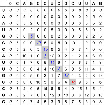 |
| Figure 13.1
Similarity table and best alignment for two small sequences CAGCCUCGCUUAG (top) and AAUGCCAUUGCCGG (left).The best alignment is highlighted in light gray values terminated by the Bold value (maximal) score.
|
 |
| Figure 13.2
Dependency of the values in the Smith-Waterman table. The gray values in the tables determine the value in the lower right corner.
|
Prior work on GPUs has focused on problems that involve solving many independent SW problems. For example the Swiss-Prot protein database (release 56.6) consists of 405,506 separate protein sequences. The proteins in this database have an average sequence length of 360 amino acids each. In this type of alignment problem, it is possible to perform many separate SW tests in parallel (one for each of the many proteins). Each thread (or sometimes a thread block) independently calculates a separate table. Performing many separate SW problems is a static load-balancing problem because the many problems are different sizes. But having many separate problems to work on removes the dependency issue.
However, in this work we wish to solve a single large SW problem. For example, each human chromosome contains on the order of
 nucleic acid base pairs. When one is interested in the interstitial sequences between the active genes, there are no clear breaks in this sequence, and it must be searched in its entirety. Similarly, searching a voice sequence for a particular word generally requires searching the entire voice stream (also roughly
 long) in its entirety.
13.3. Algorithms, Implementations, and Evaluations
There are a number of optimizations to the SW algorithm that are relevant to this discussion. They are detailed in the next sections.
13.3.1. Reduced Dependency
The dependency requirements (and work) of the SW algorithm can be significantly reduced at the expense of using additional memory by using the three-variable formula,
 where
where
 is the modified row maximum and
 is the modified column maximum. The dependencies for this algorithm are shown in
Figure 13.3
.
Figure 13.3
shows the
is the modified column maximum. The dependencies for this algorithm are shown in
Figure 13.3
.
Figure 13.3
shows the
 values for the table, but each
table entry now actually stores a triplet of values (
values for the table, but each
table entry now actually stores a triplet of values ( ,
,
 , and
, and
 . This algorithm nominally requires reading five items and writing three items for every cell update. The five additions and three
Max
operations are very fast compared with the memory operations, so the SW algorithm is typically memory bound.
. This algorithm nominally requires reading five items and writing three items for every cell update. The five additions and three
Max
operations are very fast compared with the memory operations, so the SW algorithm is typically memory bound.
 |
| Figure 13.3
Dependencies in the three-variable Smith-Waterman table. The gray values in the tables determine the value in the lower right corner.
|
13.3.2. Antidiagonal Approach
The SW algorithm can be parallelized by operating along the antidiagonal.
Figure 13.4
shows (in gray) the cells that can be updated in parallel. If the three-variable approach is used, then the entire table does not need to be stored. An antidiagonal row can be updated from the previous
 and
and
 antidiagonal row, and the previous two antidiagonal rows of
 . The algorithm can then store the
 and
and
 location of the maximum
 value so far. When the entire table has been searched, it is then possible to return to the maximum location and rebuild the small portion of the table necessary to reconstruct the alignment subsequences.
 |
| Figure 13.4
Antidiagonal parallelism. All the question table entries can be computed in parallel, using the prior two antidiagonals and the sequence data.
|
The antidiagonal method has start-up and shut-down issues that make it somewhat unattractive to program. It is inefficient (by a factor of roughly 50%) if the two input sequences have similar sizes. For very dissimilar sized input sequences, the maximum length of the antidiagonal row is the minimum of the two input sequence lengths. On a GPU we would like to operate with roughly 128 to 256 threads
per block and at least two blocks per multiprocessor (32-60 blocks). This means that we need query sequences of length
 or greater to efficiently occupy the GPU using the antidiagonal method. This is an order of magnitude larger than a typical query sequence.
The antidiagonal method can not operate entirely with just registers and shared memory. The inherent algorithm dependencies still require extensive communication of the values of
 ,
,
 , and
, and
 between the threads.
13.3.3. Row (or Column) Parallel Approach
If a parallel scan is used, the SW algorithm can be parallelized along rows or columns
[3]
. The row/column parallel algorithm takes three steps. The first step involves a temporary variable,
 . A row of
 is computed in parallel from previous row data via
 The variable
 is then used instead of
 and is given by
 which can be computed efficiently using a modified parallel maximum scan of the previous
 row. Finally, the values of H are computed in parallel for the new row using the expression

In this algorithm the first step and the last steps are entirely local. Data from a different thread is not required. The dependency problem is forced entirely into the parallel scan. Efficient methods to perform this scan on the GPU are well understood. We simply need to modify them slightly to account for the gap extension penalty
 . These code modifications are presented in the Appendix. The row parallel SW algorithm is also attractive on GPUs because it leads to sequential coalesced memory accesses. One row of the calculation is shown in
Figure 13.5
.
. These code modifications are presented in the Appendix. The row parallel SW algorithm is also attractive on GPUs because it leads to sequential coalesced memory accesses. One row of the calculation is shown in
Figure 13.5
.
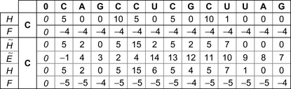 |
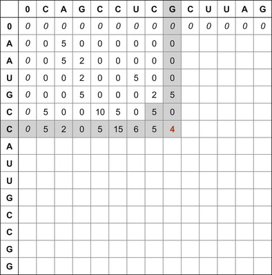
| Figure 13.5
An example of the calculations in a row-parallel scan Smith-Waterman algorithm. This example is calculating the sixth row from the fifth row data (of the example problem shown in
Figure 13.1
).
|
The parallel scan can be adapted to work on many GPUs. It requires sending one real number from each GPU in the middle of the scan (between the up and the down sweeps of the scan algorithm). The results presented in this chapter do not use this approach. Although the amount of data being sent is small, this approach still produces a synchronization point between the GPUs that can
reduce the parallel efficiency. Instead, the idea of overlapping, described next, is used for the inter-GPU parallelism.
13.3.4. Overlapping Search
If an upper bound is known a priori for the length of the alignment subsequences that will result from the search, it is possible to start the SW search algorithm somewhere in the middle of the table. This allows an entirely different approach to parallelism.
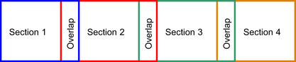
Figure 13.6
shows an example where the database sequence has been broken into four overlapping parts. If the region of overlap is wider than any subsequence that is found, then each part of the database can be searched independently. The algorithm will start each of the four searches with zeros in the left column. This is correct for the first section, but not for the other sections. Nevertheless, by the time that the end of the overlap region has been reached, the table values computed by the other sections will be the correct values.
 |
| Figure 13.6
Example of the overlapping approach to parallelism.
|
This means that in the overlap region the values computed from the section on the overlap region's left are the correct values. The values computed at the beginning of the section that extends to the right are incorrect and are ignored (in the overlap region) for the purposes of determining best alignment subsequences.
This approach to parallelism is attractive for partitioning the problem onto the different GPUs. It does not require any communication at all between the GPUs except a transfer of the overlapping part of the database sequence at the beginning of the computation and a collection (and sorting) of the best alignments at the very end. This approach also partitions a large database into much more easily handled/accessed database sections. The cost to be paid lies in the duplicate computation that is occurring in the overlap regions and the fact that the amount of overlap must be estimated before the computation occurs.
For a
 long database on 100 GPUs, each GPU handles a database section of a million items. If the expected subsequence alignments are less than
 long, the overlap is less than 1% of the total computation. However, if we were to try to extend this approach to produce parallelism at the block level (with 100 blocks on each GPU), the amount of overlap being computed would be 100%, which would be quite inefficient. Thread-level parallelism using this approach (assuming 128 threads per block and no more than 10% overlap) would require that subsequences be guaranteed to be less than eight items long. This is far too small, so thread-level parallelism is not possible using overlapping. The approach used in this chapter, which only uses overlapping at the GPU level, can efficiently handle potential subsequence alignments that are comparable to the size of the database section being computed on each GPU (sizes up to
 in our current example). For larger alignments, the GPU parallel scan would be necessary.
13.3.5. Data Packing
Because the SW algorithm is memory constrained, one simple method to improve the performance significantly is to pack the sequence data and the intermediate table values. For example, when one is working with DNA or RNA sequences, there are only four possibilities (2 bits) for each item in the sequence. Sixteen RNA items can therefore be stored in a single 32-bit integer, increasing the performance of the memory reads to the sequence data by a factor of 16. Similarly, for protein problems 5 bits are sufficient to represent one amino acid resulting in 6 amino acids per 32-bit integer read (or write).
The bits required for the table values are limited by the maximum expected length of the subsequence alignments and by the similarity scoring system used for a particular problem. The Scalable Synthetic Compact Application (SSCA) No. 1 benchmark sets the similarity value to 5 for a match, so the maximum table values will be less than or equal to 5* (the alignment length). Therefore, 16 bits are sufficient for sequences of length up to
 .
.
Data packing is problem dependent, so we have not implemented it in our code distribution (web site), or used it to improve the speed of the results presented in the subsequent sections.
13.3.6. Hash Tables
Some commonly used SW derivatives (such as FASTA and BLAST) use heuristics to improve the search speed. One common heuristic is to insist upon perfect matching of the first
 items before a subsequence is evaluated as a potential possibility for an optimal alignment. This step and some preprocessing of the database allow the first
 items of each query sequence to be used as a hash table to reduce the search space.
For example, if the first four items are required to match perfectly, then there are 16 possibilities for the first four items. The database is then preprocessed into a linked list with 16 heads. Each linked list head points to the first location in the database of that particular four-item string, and each location in the database points to the next location of that same type.
In theory this approach can reduce the computational work by roughly a factor of 2
 . It also eliminates the optimality of the SW algorithm. If the first eight items of a 64-item final alignment must match exactly, there is roughly a 12.5% chance that the alignment found is actually suboptimal. On a single CPU, the BLAST and FASTA programs typically go about 60 times faster than optimal SW.
Because this type of optimization is very problem dependent and is difficult to parallelize, we have not included it in our code or the following results.
Lincoln is a National Science Foundation (NSF) Teragrid GPU cluster located at National Center for Supercomputing Applications (NCSA). Lincoln has 96 Tesla S1070 servers (384 Tesla GPUs). Each of Lincoln's 192 servers holds two Intel 64 (Harpertown) 2.33 GHz dual-socket quad-core processors with
 MB L2 cache and 2 GB of RAM per core. Each server CPU (with four cores) is connected to one of the Tesla GPUs via PCI-e Gen2 X8 slots. All code was written in C
 with NVIDIA's CUDA language extensions for the GPU. The results were compiled using Red Hat Enterprise Linux 4 (Linux 2.6.19) and the GCC compiler.
The SW algorithm is implemented as two kernels. The first kernel identifies the end points of the best sequence matches by constructing the SW table. This is the computationally intensive part of the algorithm. The best end-point locations are saved but not the table values. Once the best sequences end points are found (200 of them in this test), the second kernel goes back and determines the actual sequences by reconstructing small parts of the table and using a trace-back procedure. The second kernel is less amenable to efficient implementation on the GPU (we devote one GPU block to each trace-back operation), but it is also not very computationally intensive. Splitting the two tasks, rather than identifying the sequences on the fly as they are found, prevents the GPUs from getting stalled during the computationally expensive task.
Timings for five different NVIDIA GPUs and one core of an AMD CPU (quad-core Phenom II X4 CPU operating at 3.2 GHz, with
 KB of L2 cache, 6 MB of L3 cache) are shown in
Figure 13.7
. Speedups over the CPU of close to a factor of 100 can be obtained on table sizes (query sequence size times database size) that are larger than 1B. The CPU code has been compiled with optimization on (
KB of L2 cache, 6 MB of L3 cache) are shown in
Figure 13.7
. Speedups over the CPU of close to a factor of 100 can be obtained on table sizes (query sequence size times database size) that are larger than 1B. The CPU code has been compiled with optimization on ( 03), but the algorithm itself was not hand optimized (by using MMX instructions, for example).
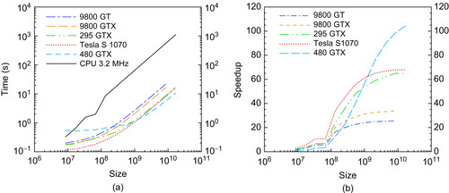 |
| Figure 13.7
Performance of a single GPU for the Smith-Waterman algorithm (kernel 1) for a test sequence of 1024 and various database sizes. The size axis refers to the total table size. (a) Time. (b) Speedup versus one core of a 3.2 GHz AMD quad-core Phenom II X4 CPU.
|
A single GPU can search for an optimal match of a 1000 long query sequence in a 1M long database in roughly 1 second. In contrast the time to determine the 200 sequences corresponding to the 200 best matches (kernel 2) is about 0.02 seconds on the CPU, and this calculation is independent of the database size. The GPUs were programmed to perform this task, but they took 0.055 seconds (for the 8800 GT) to 0.03 seconds for the 295GTX. With shorter query sequences, 128 long instead of the 512 long sequences quoted earlier in this chapter, the GPU outperforms the CPU on kernel 2 by about three times. The impact of kernel 2 on the total algorithm time is negligible in all cases.
When the problem size is held constant and the number of processors is varied, we obtain strong scaling results.
Figure 13.8
shows the speedup obtained when a 16M long database is searched with a 128 long query sequence on Lincoln. Ideally, the speedup in this case should be linear with the number of GPUs. In practice, as the number of GPUs increases, the problem size per GPU decreases, and small problem sizes are less efficient on the GPU. When 120 GPUs are working on this problem, each GPU is only constructing a subtable of roughly size
 . From
Figure 13.7
it is clear that this size is an order of magnitude too small to be reasonably efficient on the GPU.
. From
Figure 13.7
it is clear that this size is an order of magnitude too small to be reasonably efficient on the GPU.
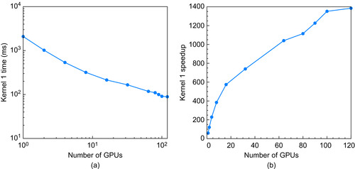 |
| Figure 13.8
Strong scaling timings with 16 M for database and 128 for test sequence. (a) Time. (b) Speedup versus one core of a 3.2 GHz AMD quad-core Phenom II X4 CPU.
|
Weak scaling allows the problem size to grow proportionally with the number of GPUs so that the work per GPU remains constant. The cell updates per second (GCUPS) for this weak-scaled problem are shown in
Figure 13.9a
, when 2M elements per GPU are used for the database size, and a 128-element query sequence is used. Because the amount of work being performed increases proportionally with the number of GPUs used, the GCUPS should be linear as the number of GPUs is increased. However, the time increases slightly because of the increased communication burden between GPUs as their number is increased. The total time varies from 270 ms to 350 ms, and it increases fairly slowly with the number of GPUs used.
Figure 13.9b
shows speedups for kernel 1 on the Lincoln supercomputer
compared with a single-CPU core of an AMD quad-core. Compared with a single CPU core, the speedup is almost 56x, for a single GPU, and 5335x, for 120 GPUs (44x faster per GPU).
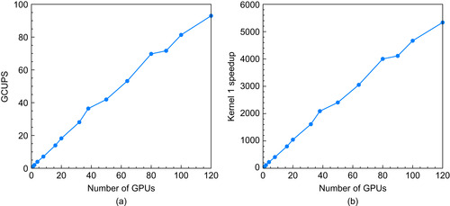 |
| Figure 13.9
Weak scaling GCUPS (a) and speedups (b) for kernel 1 using various numbers of GPUs on Lincoln with 2M elements per GPU for the database size and a 128-element test sequence.
|
The current implementation keeps track of the location of the highest 200 alignment scores on each GPU. This list changes dynamically as the algorithm processes the rows of the table. The first few rows cause many changes to this list. The changes are then less frequent, but still require continual sorting of the list. This portion of the code takes about 2% of the total time. The breakdown for the other three steps of the algorithm is shown in
Table 13.1
.
| Top 200 | Scan for
| |||
|---|---|---|---|---|
| 295 GTX | 2% | 30% | 48% | 20% |
| 480 GTX | 3% | 27% | 54% | 16% |
The scan is the most expensive part of the three steps. This scan was adapted from an SDK distribution that accounts for bank conflicts and is probably performing at close to the peak possible efficiency. If a single SW problem is being solved on the GPU, then the problem is inherently coupled. The row-parallel algorithm isolates the dependencies in the Smith-Waterman problem as much as is possible, and solves for those dependencies as efficiently as possible, using the parallel scan.
The maximum memory bandwidth that can be achieved on Lincoln is close to 85 GB/s for a single GPU. Based on our algorithm (7 memory accesses per cell) the maximum theoretical GCUPS is close to 3.0 (85/4/7) for a single GPU. Since this code obtains 1.04 GCUPS per GPU, the algorithm is
reasonably efficient (34% of the peak memory throughput). Higher GCUPS rates for a single GPU would be possible by using problem dependent optimizations such as data packing or hash tables.
The row parallel algorithm doesn't have any limitation on the query or database sequence sizes. For example, a database length of 4M per GPU was compared with a query sequence of 1M. This query took 4229 seconds on Lincoln and 2748 seconds on the 480 GTX. This works out to 1.03 and 1.6 GCUPS per GPU for the Tesla S1070 and 480 GTX GPUs respectively. This is very similar to the performance obtained for smaller test sequences, because the algorithm works row by row and is therefore independent of the number of rows (which equals the query or test sequence size).
13.5. Future Direction
One way to optimize this algorithm further is to combine the three steps into a single GPU call. The key to this approach is being able to synchronize the threads within the kernel, because each step of the algorithm must be entirely completed (for all threads) before the next step can be executed. The first synchronization point is after finishing the up-sweep step of the parallel scan, and second one is after finding the value for
 . At both GPU synchronization points one number per block must be written to the global memory. All other data items are then kept in the shared memory (it is possible to use registers for some data), so the number of access to the global memory is reduced to 3 per cell update. Early indications have been that within experimental error, this approach is not faster than the approach of issuing separate GPU kernel calls to enforce synchronization of the threads.
Because the algorithm operates row-by-row the query size (number of rows) is entirely arbitrary and limited only by the patience of the user. In contrast, the database size is restricted by the total memory available from all the GPUs (so less than
 when using 100 Tesla GPUs). In practice human patience expires before the database memory is exhausted.
Acknowledgments
This work was supported by the Department of Defense and used resources from the Extreme Scale Systems Center at Oak Ridge National Laboratory. Some of this work occurred on the NSF Teragrid supercomputer, Lincoln, located at NCSA.
Appendix
The most important part of a row parallel approach for the GPU is the contiguous and coalesced access to the memory that this algorithm allows and the fact that the level of small-scale parallelism is now equal to the
maximum
of the query sequence and the database lengths.
Each step of the row parallel approach can be optimized for the GPU. In the first step (when calculating
 , two
, two
 values are needed (
 . To enable coalesced memory accesses and minimize accesses to the global memory,
 values are first copied to the shared memory. The second step of the algorithm (that calculates the
 uses a modification of the
scanLargeArray
code found
in the SDK of CUDA 2.2. This code implements a work-efficient parallel sum scan
[4]
. The work-efficient parallel scan has two sweeps, an Up-Sweep and a Down-Sweep. The formulas for the original Up-sweep sum scan (from the SDK) and for our modified scan are shown at the end of this paragraph. The major change is to change the sum to a max, and then to modify the max arguments (terms in bold).
uses a modification of the
scanLargeArray
code found
in the SDK of CUDA 2.2. This code implements a work-efficient parallel sum scan
[4]
. The work-efficient parallel scan has two sweeps, an Up-Sweep and a Down-Sweep. The formulas for the original Up-sweep sum scan (from the SDK) and for our modified scan are shown at the end of this paragraph. The major change is to change the sum to a max, and then to modify the max arguments (terms in bold).
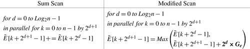 |
The formulas for down-sweep for both scans are
 |
Detailed implementation of these scan algorithms is presented in reference
[5]
. This reference explains how this algorithm uses shared memory and avoids bank conflicts. In the
scanLargeArray
code in the SDK, the scan process is recursive. The values in each block are scanned individually and then are corrected by adding the sum from the previous block (this is the
uniformAdd
kernel in the SDK). Our implementation does not perform this last step of the scan. Instead, every block needs the scan result from the previous block (we assume that no alignment sequence has a gap length greater than 1024 within it). Before putting zero in the down-sweep scan for the last element, we save this final number (one for each block) in global memory, and the next block uses this number instead of forcing it to be zero. Only the first block uses zero; the other blocks use the previous block's result.
If one needed to assume gaps greater than 1024 are possible, it is not difficult to modify the existing scan code.
uniformAdd
would need to be replaced with a
uniformMax
subroutine. This would save the last number at the end of the up-sweep,
 . The new value of
 is related to the number of threads in a block and the level of the recursive scan call. For example, if one uses 512 threads per block for the scan, then
 Then in
uniformMax
, the correction is given by
Then in
uniformMax
, the correction is given by
 where
where
 is the result of the block scan and
 is the previous gap extension penalty. This
uniformMax
subroutine must be applied to all the elements. In our test cases,
uniformMax
would never cause any change in the results (because all sequences have far fewer than 1024 gaps). The
Max
always returns the first argument.
is the previous gap extension penalty. This
uniformMax
subroutine must be applied to all the elements. In our test cases,
uniformMax
would never cause any change in the results (because all sequences have far fewer than 1024 gaps). The
Max
always returns the first argument.
After the 200 best alignments in kernel 1 are found, sequence extraction is done in kernel 2 with each thread block receiving one sequence end point to trace back. By starting from the end point and constructing the similarity table backward for a short distance, one can actually extract the sequences. For kernel 2 the antidiagonal method is used within each thread block. Because the time is small for kernel 2 and because this kernel is not sensitive to the length of the database, global memory was used. The trace back procedure is summarized below.

References
[1]
Y. Liu, B. Schmidt, D.L Maskell,
CUDASW++2.0: enhanced Smith-Waterman protein database search on CUDA-enabled GPUs based on SIMT and virtualized SIMD abstractions
,
BMC Res.
Notes 3
(2010
)
93
.
[2]
L. Ligowski, W. Rudnicki,
An efficient implementation of Smith Waterman algorithm on GPU using CUDA, for massively parallel scanning of sequence databases
,
In:
23rd IEEE International Parallel and Distributed Processing Symposium, May 25–29
(2009
)
Aurelia Convention Centre & Expo Rome
,
Italy
.
[3]
A. Khajeh-Saeed, S. Poole, J.B. Perot,
Acceleration of the Smith–Waterman algorithm using single and multiple graphics processors
,
J. Comput. Phys.
229
(2010
)
4247
–
4258
.
[4]
M. Harris, S. Sengupta, J.D. Owens,
Parallel prefix sum (scan) with CUDA
,
In:
GPU Gems 3, Chapter 39
(December 2007
)
NVIDIA Corporation
,
USA
.
[5]
S. Sengupta, M. Harris, Y. Zhang, J.D. Owens,
Scan primitives for GPU computing
,
In:
Graph
(August 4–5, 2007
)
Hardware 2007
,
San Diego, CA
.
..................Content has been hidden....................
You can't read the all page of ebook, please click here login for view all page.