
Chapter 15. Temporal Data Mining for Neuroscience
Wu-chun Feng, Yong Cao, Debprakash Patnaik and Naren Ramakrishnan
Today, multielectrode arrays (MEAs) capture neuronal spike streams in real time, thus providing dynamic perspectives into brain function. Mining such spike streams from these MEAs is critical toward understanding the firing patterns of neurons and gaining insight into the underlying cellular activity. However, the acquisition rate of neuronal data places a tremendous computational burden on the subsequent temporal data mining of these spike streams. Thus, computational neuroscience seeks innovative approaches toward tackling this problem and eventually solving it efficiently and in real time.
In this chapter, we present a solution that uses graphics processing units (GPUs) to mine spike train datasets. Specifically, our solution delivers a novel mapping of a “finite state machine for data mining” onto the GPU while simultaneously addressing a wide range of neuronal input characteristics. This solution ultimately transforms the task of temporal data mining of spike trains from a batch-oriented process towards a real-time one.
15.1. Introduction
Brain-computer interfaces have made massive strides in recent years
[1]
. Scientists are now able to analyze neuronal activity in living organisms, understand the intent implicit in these signals and, more importantly, use this information as control directives to operate external devices. Technologies for modeling and recording neuronal activity include functional magnetic resonance imaging (fMRI), electroencephalography (EEG), and multielectrode arrays (MEAs).
In this chapter, we focus on event streams gathered through MEA chips for studying neuronal function. As shown in
Figure 15.1
, an MEA records spiking action potentials from an ensemble of neurons, and after various preprocessing steps, these neurons yield a spike train dataset that provides a real-time dynamic perspective into brain function. Key problems of interest include identifying sequences of firing neurons, determining their characteristic delays, and reconstructing the functional connectivity of neuronal circuits. Addressing these problems can provide critical insights into the cellular activity recorded in the neuronal tissue.
 |
| Figure 15.1
Spike trains recorded from a multielectrode array (MEA) are mined by a GPU to yield frequent episodes, which can be summarized to reconstruct the underlying neuronal circuitry.
|
In only a
few minutes
of cortical recording, a 64-channel MEA can easily capture
millions
of neuronal spikes. In practice, such MEA experiments run for
days
or even months
[8]
and can result in
trillions
to
quadrillions
of neuronal spikes. From these neuronal spike streams, we seek to identify (or mine for)
frequent episodes
of repetitive patterns that are associated with higher-order brain function. The mining algorithms of these patterns are usually based on finite state machines
[3]
and
[5]
and can handle temporal constraints
[6]
. The temporal constraints add significant complexity to the state machine algorithms as they must now keep track of what part of an episode has been seen, which event is expected next, and when episodes interleave. Then, they must make a decision of which events to be used in the formation of an episode.
15.2. Core Methodology
We model a spike train dataset as an event stream, where each symbol/event type corresponds to a specific neuron (or clump of neurons). In addition, the dataset encodes the occurrence times of these events.
Temporal data mining of event streams aims to discover interesting patterns that occur frequently in the event stream, subject to certain timing constraints. More formally, each pattern (i.e., episode) is an ordered tuple of event types with temporal constraints. For example, the episode shown below describes a pattern where event
 must occur at least
 after event
 and at most
 after event
 and event
 must occur at least
 after event
 and at most
 after event
 .
.
 The preceding is a size-three episode because it contains three events.
Episodes are mined by a generate-and-test approach; that is, we generate numerous candidate episodes that are counted to ascertain their frequencies. This process happens levelwise: search for one-node episodes (single symbols) first, followed by two-node episodes, and so on. At each level, size-
N
candidates are generated from size-(N
) frequent episodes, and their frequencies (i.e., counts) are determined by making a pass over the event sequence. Only those candidate episodes whose count is greater than a user-defined threshold are retained. The most computationally expensive step in each level is the counting of all candidate episodes for that level. At the initial levels, there are a large number of candidate episodes to be counted in parallel; the later levels only have increasingly fewer candidate episodes.
The frequency of an episode is a measure that is open to multiple interpretations. Note that episodes can have “junk” symbols interspersed; for example, an occurrence of event A followed by B followed by C might have symbol D interspersed, whereas a different occurrence of the same episode might have symbol F interspersed. Example ways to define frequency include counting all occurrences, counting only nonoverlapped occurrences, and so on. We utilize the nonoverlapped count, which is defined as the maximum number of nonoverlapped instances of the given episode. This measure has the advantageous property of
antimonotonicity
; that is, the frequency of a subepisode cannot be less than the frequency of the given episode. Antimonotonicty allows us to use levelwise pruning algorithms in our search for frequent episodes.
Our approach is based on a state machine algorithm with interevent constraints
[6]
.
Algorithm 1
shows our serial counting procedure for a single episode
 . The algorithm maintains a data structure
 , which is a list of lists. Each list
 in
in
 corresponds to an event type
 and stores the times of occurrences of those events with event type
 that satisfy the interevent constraint
 with at least one entry
 . This requirement is relaxed for
 , thus every time an event
 is seen in the data, its occurrence time is pushed into
 .
.
When an event of type
 at time
 is seen, we look for an entry
 such that
 . Therefore, if we are able to add the event to the list
 , it implies that there exists at least one previous event with event type
 in the data stream for the current event that satisfies the interevent constraint between
 and
and
 . After we apply this argument recursively, if we can add an event with event type
 to its corresponding list in
 , then there exists a sequence of events corresponding to each event type in
 satisfying the respective interevent constraints. Such an event marks the end of an occurrence, after which the
 for
for
 is incremented and the data structure
 is reinitialized.
Figure 15.2
illustrates the data structure
is reinitialized.
Figure 15.2
illustrates the data structure
 for counting
 .
.
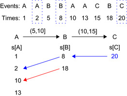 |
| Figure 15.2
An illustration of the data structure
|
Input:
Candidate
N
-node episode
 and event sequence
 .
.
Output:
Count of nonoverlapped occurrences of
 satisfying interevent constraints
1:
 ;
;
 //List of
 lists
lists
2:
for all
 do
do
3:
for
 do
do
4:
 event type of

5:
if
 then
then
6:

7:
if
 then
then
8:

9:
while
 do
do
10:

11:
if
 then
then
12:
if
 then
then
13:
 ;
;
 ;
break
Line: 1.2
;
break
Line: 1.2
14:
else
15:

16:
break
Line: 1.2
17:

18:
else
19:

20: RETURN count
15.3. GPU Parallelization: Algorithms and Implementations
To parallelize the aforementioned sequential counting approach on a GPU, we segment the overall computation into independent units that can be mapped onto GPU cores and executed in parallel to
fully utilize GPU resources. Different computation-to-core mapping schemes can result in different levels of parallelism, which are suitable for different inputs for the episode counting algorithm. Next, we present two computation-to-core mapping strategies, which are suitable for different scenarios with different sizes of input episodes. The first strategy, one thread per occurrence of an episode, is used for mining a very few episodes. The second strategy is used for counting many episodes.
15.3.1. Strategy 1: One Thread per Occurrence
Problem Context
This mapping strategy handles the case when we have a few input episodes to count. In the limit, mining one episode with one thread severely underutilizes the GPU. Thus, we seek an approach to increase the level of parallelism. The original sequential version of the mining algorithm uses a state-machine approach with a substantial amount of data dependencies. Hence, it is difficult to increase the degree of parallelism by optimizing this algorithm directly. Instead, we transform the algorithm by discarding the state-machine approach and decomposing the problem into two subproblems that can be easily parallelized using known computing primitives. The mining of an episode entails counting the frequency of nonoverlapped neuronal patterns of event symbols. It represents the size of the largest set of nonoverlapped occurrences. Based on this definition, we design a more data-parallel solution.
Basic Idea
In our new approach, we find a superset of the nonoverlapped occurrences that could potentially be overlapping. Each occurrence of an episode has a start time and an end time. If each episode occurrence in this superset is viewed as a task/job with fixed start and end times, then the problem of finding the largest set of nonoverlapped occurrences transforms itself into a job-scheduling problem, where the goal is to maximize the number of jobs or tasks while avoiding conflicts. A greedy
 algorithm solves this problem optimally where
 is the number of jobs. The original problem now decomposes into two subproblems:
1. Find a superset of nonoverlapped occurrences of an episode
2. Find the size of the largest set of nonoverlapped occurrences from the set of occurrences
The first subproblem can be solved with a high degree of parallelism as will be shown later in this chapter. We design a solution where one GPU thread can mine one occurrence of an episode. To preprocess the data, however, we perform an important compaction step between the searches of the next query event in the episode. This entailed us to investigate both a lock-based compaction method using atomic operations in CUDA as well as a lock-free approach with the CUDPP library. However, the performance of both compaction methods was unsatisfactory. Thus, in order to further improve performance, we adopted a counterintuitive approach that divided the counting process into three parts. First, each thread looks up the event sequence for suitable next events, but instead of recording the events found, it merely counts and writes the count to global memory. Second, an exclusive scan is performed on the recorded counts. This gives the offset into the global memory where each thread can write its “next events” list. The actual writing is done as the third step. Although each thread looks up the event sequence twice (first to count and second to write), we show that we nevertheless achieve better performance.
Algorithmic Improvements
We first preprocess the entire event stream, noting the positions of events of each event type. Then, for a given episode, beginning with the list of occurrences of the start event type in the episode, we find occurrences satisfying the temporal constraints in parallel. Finally, we collect and remove overlapped occurrences in one pass. The greedy algorithm for removing overlaps requires the occurrences to be sorted by end time, and the algorithm proceeds as shown in
Algorithm 2
. Here, for every set of consecutive occurrences, if the start time is after the end time of the last selected occurrence, then we select this occurrence; otherwise, we skip it and go to the next occurrence.
Next, we explore different approaches of solving the first subproblem, as presented earlier. The aim here is to find a superset of nonoverlapped occurrences in parallel. The basic idea is to start with all events of the first event-type in parallel for a given episode and find occurrences of the episode starting at each of these events. There can be several different ways in which this can be done. We shall present two approaches that showed the most performance improvement. We shall use the episode
 as our running example and explain each of the counting strategies using this example. This example episode specifies event occurrences where an event
 is to be followed by an event
 within 5–10 ms and event
 is to be followed by an event
 within 5–10 ms delay. Note again that the delays have both a lower and an upper bound.
Parallel Local Tracking
In the preprocessing step, we have noted the locations of each of the event-types in the data. In the counting step, we launch as many threads as there are events in the event stream of the start event type (of the episode). In our running example these are all events of type
 . Each thread searches the event stream starting at one of these events of type
 and looks for an event of type
 that satisfies the inter event time constraint
 ; that is,
 where
where
 are the indices of the events of type
 and
and
 . One thread can find multiple
 's for the same
 . These are recorded in a preallocated array assigned to each thread. Once all the events of type
 (with an
 before them) have been collected by the threads (in parallel), we need to compact these newfound events into a contiguous array/list. This is necessary because in the next kernel launch we will find all the events of type
 that satisfy the interevent constraints with this set of
 's. This is illustrated in
Figure 15.3
.
's. This is illustrated in
Figure 15.3
.
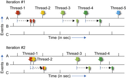 |
| Figure 15.3
Illustration of the parallel local tracking algorithm (i.e.,
Algorithm 3
), showing two iterations for the episode
|
Input:
Iteration number
 , Episode
 ,
,
 :
:
 event-type in
 , Index list
 , Data sequence
 .
.
Output:
 : Indices of events of type
 .
.
for all
threads with distinct identifiers
 do
do
Scan
 starting at event
 for event-type
 satisfying inter-event constraint
 .
.
Record all such events of type
 .
.
Compact all found events into the list
 .
.

Algorithm 3
presents the work done in each kernel launch. In order to obtain the complete set of occurrences of an episode, we need to launch the kernel
 times where
 is the size of an episode. The list of qualifying events found in the
 iteration is passed as input to the next iteration. Some amount of bookkeeping is also done to keep track of the start and end times of an occurrence. After this phase of parallel local tracking is completed, the nonoverlapped count is obtained using
Algorithm 2
. The compaction step in
Algorithm 3
presents a challenge because it requires concurrent updates into a global array.
iteration is passed as input to the next iteration. Some amount of bookkeeping is also done to keep track of the start and end times of an occurrence. After this phase of parallel local tracking is completed, the nonoverlapped count is obtained using
Algorithm 2
. The compaction step in
Algorithm 3
presents a challenge because it requires concurrent updates into a global array.
Implementation Notes
Lock-Based Compaction
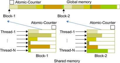
NVIDIA graphics cards with CUDA compute capability 1.3 support atomic operations on shared and global memory. Here, we use atomic operations to perform compaction of the output array into the global memory. After the counting step, each thread has a list of next events. Subsequently, each thread adds the size of its next events list to the block-level counter using an atomic add operation and, in
return, obtains a local offset (which is the previous value of the block-level counter). After all threads in a block have updated the block-level counter, one thread from a block updates the global counter by adding the value of the block-level counter to it and, as before, obtains the offset into global memory. Now, all threads in the block can collaboratively write into the correct position in the global memory (resulting in overall compaction). A schematic for this operation is shown for two blocks in
Figure 15.4
. In the results section, we refer to this method as
AtomicCompact
.
 |
| Figure 15.4
Illustration of output compaction using atomicAdd operations. Note that we use atomic operations at both block and global level. These operations return the correct offset into global memory for each thread to write its next-event list into.
|
Because there is no guarantee for the order of atomic operations, this procedure requires sorting. The complete occurrences need to be sorted by end time for
Algorithm 2
to produce the correct result.
Lock-Free Compaction
Prefix scan is known to be a general-purpose, data-parallel primitive that is a useful building block for algorithms in a broad range of applications. Given a vector of data elements
 , an associative binary function
 and an identity element
 , exclusive prefix scan returns
 . The first parallel prefix-scan algorithm was proposed in 1962
[4]
. With increasing interest in general-purpose computing on the GPU (GPGPU), several implementations of scan algorithms have been proposed for the GPU, the most recent ones being
[2]
and
[7]
. The latter implementation is available as the
CUDPP: CUDA Data Parallel Primitives Library
and forms part of the CUDA SDK distribution.
. The first parallel prefix-scan algorithm was proposed in 1962
[4]
. With increasing interest in general-purpose computing on the GPU (GPGPU), several implementations of scan algorithms have been proposed for the GPU, the most recent ones being
[2]
and
[7]
. The latter implementation is available as the
CUDPP: CUDA Data Parallel Primitives Library
and forms part of the CUDA SDK distribution.
Our lock-free compaction is based on prefix sum, and we reuse the implementation from the CUDPP library. Because the scan-based operation guarantees ordering, we modify our counting procedure to count occurrences backward starting from the last event. This results in the final set of occurrences to be automatically ordered by end time and therefore completely eliminates the need for sorting (as required by the approach based on atomic operations).
The CUDPP library provides a compact function that takes an array
 , an array of
 flags, and returns a compacted array
d
out
of corresponding only the “valid” values from
flags, and returns a compacted array
d
out
of corresponding only the “valid” values from
 (it internally uses
cudppScan
). In order to use this, our counting kernel is now split into three kernel calls. Each thread
is allocated a fixed portion of a larger array in global memory for its next events list. In the first kernel, each thread finds its events and fills up its next-events list in global memory. The
cudppCompact
function, implemented as two GPU kernel calls, compacts the large array to obtain the global list of next-events. A difficulty of this approach is that the array on which
cudppCompact
operates is very large, resulting in a scattered memory access pattern. We refer to this method as
CudppCompact
.
(it internally uses
cudppScan
). In order to use this, our counting kernel is now split into three kernel calls. Each thread
is allocated a fixed portion of a larger array in global memory for its next events list. In the first kernel, each thread finds its events and fills up its next-events list in global memory. The
cudppCompact
function, implemented as two GPU kernel calls, compacts the large array to obtain the global list of next-events. A difficulty of this approach is that the array on which
cudppCompact
operates is very large, resulting in a scattered memory access pattern. We refer to this method as
CudppCompact
.
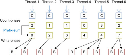
In order to further improve performance, we adopt a counterintuitive approach. We again divide the counting process into three parts. First, each thread looks up the event sequence for suitable next events but instead of recording the events found, it merely counts and writes the count to global memory. Then, an exclusive scan is performed on the recorded counts. This gives the offset into the global memory where each thread can write its next-events list. The actual writing is done as the third step. Although each thread looks up the event sequence twice (first to count, and second to write), we show that we nevertheless achieve better performance. This entire procedure is illustrated in
Figure 15.5
. We refer to this method of compaction as
CountScanWrite
in the ensuing results section.
 |
| Figure 15.5
An illustration of output compaction using the scan primitive. Each iteration is broken into three kernel calls: Counting the number of next events, using scan to compute offset into global memory, and finally launching count-procedure again but this time allowing write operations to the global memory.
|
Note that prefix scan is essentially a sequential operator applied from left to right to an array. Hence, the memory writes operations into memory locations generated by prefix scan preserve order. The sorting step (i.e., sorting occurrences by end time) required in the lock-based compaction can be completely avoided by counting occurrences backward, starting from the last event type in the episode.
15.3.2. Strategy 2: A Two-Pass Elimination Approach
Problem Context
When mining a large number of input episodes, we can simply assign one GPU thread for each episode. Because there are enough episodes, the GPU computing resource will be fully utilized. The state-machine-based algorithm is very complex and requires a large amount of shared memory and a large number of GPU registers for each GPU thread. For example, if the length of the query is 5, each thread requires 220 bytes of shared memory and 97 bytes of register file. It means that only 32 threads can be allocated on a GPU multiprocessor, which has 16 kB of shared memory and register file. As each thread
requires more resources, fewer threads can run on GPU at the same time, resulting in longer execution time for each thread.
Basic Idea
To address this problem, we sought to reduce the complexity of the algorithm without losing correctness. Our idea was to use a simpler algorithm that we call
PreElim
to eliminate most of the nonsupported episodes, and only use the more complex algorithm to determine if the rest of the episode is supported or not. To introduce the algorithm
PreElim
, we consider the solution to a slightly relaxed problem, which plays an important role in our two-pass elimination approach. In this approach, algorithm
PreElim
is simpler and runs faster than the more complex algorithm because it reduces the time complexity of the interevent constraint. As a result, when the number of episodes is very large and the number of episodes culled in the first pass is also large, the performance of our two-pass elimination algorithm is significantly better than the more complex original algorithm.
Algorithmic Improvements
Let us consider a constrained version of Problem 1. Instead of enforcing both lower limits and upper limits on interevent constraints, we design a counting solution that enforces only upper limits.
Let
 be an episode with the same event types as in
 , where
 uses the original episode definition from Problem 1. The lower bounds on the interevent constraints in
 are relaxed for
 as shown here.
(15.1)
Observation 1
In
Algorithm 1
, if lower-bounds of interevent constraints in episode
 are relaxed as
 , the list size of
 can be reduced to 1.
Proof
In
Algorithm 1
, when an event of type
 is seen at time
 while going down the event sequence,
 is looked up for at least one
 , such that
 . Note that
 represents the
 entry of
 corresponding the
 event-type in
 .
.
Let
 and
and
 be the first entry that satisfies the interevent constraint
 , i.e.,
 Also
Eq. 15.3
below follows from the fact that
Also
Eq. 15.3
below follows from the fact that
 is the first entry in
 matching the time constraint.
 From
Eq. 15.2
and
Eq. 15.3
,
Eq. 15.4
follows.
From
Eq. 15.2
and
Eq. 15.3
,
Eq. 15.4
follows.
(15.2)
(15.3)
(15.4)
This shows that every entry in
 following
 also satisfies the interevent constraint. This follows from the relaxation of the lower bound. Therefore, it is sufficient to keep only the latest time stamp
 only in
 because it can serve the purpose for itself and all entries above/before it, thus reducing
 to a single time stamp rather than a list (as in
Algorithm 1
).
to a single time stamp rather than a list (as in
Algorithm 1
).
Input:
Candidate episode
 is a
is a
 -node episode, event sequence
 .
.
Output:
Count of nonoverlapped occurrences of

1:
 ;
;
 //List of
 time stamps
2:
for all
 do
do
3:
for
 do
do
4:
 event type

5:
if
 then
then
6:

7:
if
 then
then
8:
if
 then
then
9:
if
 then
then
10:
 ;
;
 ;
break
Line: 1.3.2
;
break
Line: 1.3.2
11:
else
12:

13:
else
14:

15:
Output
: count
Combined Algorithm: Two-Pass Elimination.
Now, we can return to the original mining problem (with both upper and lower bounds). By combining Algorithm
PreElim
with our hybrid algorithm, we can develop a two-pass elimination approach that can deal with the cases on which the hybrid algorithm cannot be executed. The two-pass elimination algorithm is as follows:
1: (First pass) For each episode
 , run
PreElim
on its less-constrained counterpart,
, run
PreElim
on its less-constrained counterpart,
 .
.
2: Eliminate every episode
 , if
, if
 , where
 is the support count threshold.
3: (Second Pass) Run the hybrid algorithm on each remaining episode,
 , with both interevent constraints enforced.
The two-pass elimination algorithm yields the correct solution for Problem 1. Although the set of episodes mined under the less constrained version are not a superset of those mined under the original problem definition, we can show the following result:
 , i.e., the count obtained from Algorithm
PreElim
is an upper-bound on the count obtained from the hybrid algorithm.
, i.e., the count obtained from Algorithm
PreElim
is an upper-bound on the count obtained from the hybrid algorithm.
Theorem 1
Proof
Let
 be an occurrence of
 . Note that
 is a map from event types in
 to events in the data sequence
 . Let the time stamps for each event type in
 be
be
 . Since
 is an occurrence of
 , it follows
that
, it follows
that
 Note that
 . The inequality in
Eq. 15.5
still holds after we replace
. The inequality in
Eq. 15.5
still holds after we replace
 with
with
 to get
Eq. 15.6
.
to get
Eq. 15.6
.
 The preceding corresponds to the relaxed interevent constraint in
 . Therefore, every occurrence of
 is also an occurrence of
 , but the opposite may not be true. Hence, we have that
 .
.
(15.5)
(15.6)
In our two-pass elimination approach, algorithm
PreElim
is less complex and runs faster than the hybrid algorithm because it reduces the time complexity of the interevent constraint check from
 to
to
 . Therefore, the performance of the two-pass elimination algorithm is significantly better than the hybrid algorithm when the number of episodes is very large and the number of episodes culled in the first pass is also large, as shown by our experimental results described next.
15.4. Experimental Results
15.4.1. Datasets and Testbed
Our datasets are drawn from both mathematical models of spiking neurons as well as real datasets gathered by Wagenar
et al.
[8]
in their analysis of cortical cultures. Both these sources of data are described in detail in
[6]
. The mathematical model involves 26 neurons (event types) whose activity is modeled via inhomogeneous Poisson processes. Each neuron has a basal firing rate of 20 Hz and two causal chains of connections — one short and one long — are embedded in the data. This dataset (Sym26
) involves 60 seconds with 50,000 events. The real datasets (2-1-33, 2-1-34, 2-1-35
) observe dissociated cultures on days 33, 34, and 35 from over five weeks of development. The original goal of this study was to characterize bursty behavior of neurons during development.
We evaluated the performance of our GPU algorithms on a machine equipped with Intel Core 2 Quad 2.33 GHz and 4 GB of system memory. We used a NVIDIA GTX280 GPU, which has 240 processor cores with a 1.3 GHz clock for each core and 1 GB of device memory.
15.4.2. Performance of the One Thread per Occurrence
The best GPU implementation is compared with the CPU by counting a single episode. This is the case where the GPU was weakest in previous attempts, owing to the lack of parallelization when the episodes are few.
In terms of the performance of our best GPU method, we achieve a 6x speedup over the CPU implementation on the largest dataset, as shown in
Figure 15.6
.
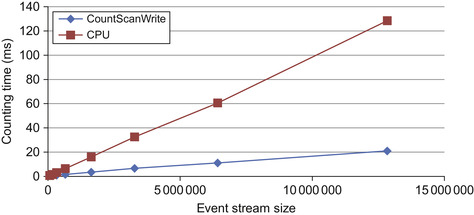 |
| Figure 15.6
Performance comparison of the CPU and best GPU implementation, counting a single episode in datasets 1 through 8.
|
Figure 15.7
contains the timing information of three compaction methods of our redesigned GPU algorithm with varying episode length. Compaction using CUDPP is the slowest of the GPU implementations, owing to its method of compaction. It requires each data element to be either in or out of the final compaction and does not allow for compaction of groups of elements. For small episode lengths, the
CountScanWrite
approach is best because sorting can be completely avoided. However, with longer episode lengths, compaction using lock-based operators shows the best performance. This method of
compaction avoids the need to perform a scan and a write at each iteration, at the cost of sorting the elements at the end. The execution time of the
AtomicCompact
is nearly unaffected by episode length, which seems counterintuitive because each level requires a kernel launch. However, each iteration also decreases the total number of episodes to sort and schedule at the end of the algorithm. Therefore, the cost of extra kernel invocations is offset by the final number of potential episodes to sort and schedule.
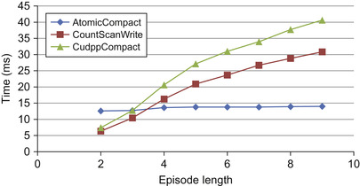 |
| Figure 15.7
Performance of algorithms with varying episode length in dataset 1.
|
We find that counting time is related to episode frequency, as shown in
Figure 15.8
. There is a linear trend, with episodes of higher frequency requiring more counting time. The lock-free compaction methods follow an expected trend of slowly increasing running time because there are more potential episodes to track. The method that exhibits an odd trend is the lock-based compaction,
AtomicCompact
. As the frequency of the episode increases, there are more potential episodes to sort and schedule. The running time of the method becomes dominated by the sorting time as the episode frequency increases.
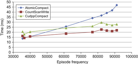 |
| Figure 15.8
Performance of algorithms with varying episode frequency in dataset 1.
|
Another feature of
Figure 15.8
that requires explanation is the bump where the episode frequency is slightly greater than 80,000. This is because it is not the final nonoverlapped count that affects the running time; it is the total number of overlapped episodes found before the scheduling algorithm is applied to remove overlaps. The x-axis is displaying nonoverlapped episode frequency, where the runtime is actually affected more by the overlapped episode frequency.
We used the CUDA Visual Profiler on the other GPU methods. They had similar profiler results as the
CountScanWrite
method. The reason is that the only bad behavior exhibited by the method is divergent branching, which comes from the tracking step. This tracking step is common to all of the GPU methods of the redesigned algorithm.
15.4.3. Performance of the Two-Pass Elimination Algorithm
The performance of the hybrid algorithm suffers from the requirement of large shared memory and large register file, especially when the episode size is big. So we introduce algorithm
PreElim
, which can eliminate most of the nonsupported episodes and requires much less shared memory and register file, and then the complex hybrid algorithm can be executed on much fewer episodes, resulting in performance gains. The amount of elimination that
PreElim
conducts can greatly affect the execution time at different episode sizes. In segment (a) of
Figure 15.9
, the
PreElim
algorithm eliminates over 99.9% (43,634 out of 43,656) of the episodes of size four. The end result is a speedup of
 over the hybrid algorithm for this episode size and an overall speedup for this support threshold of
 . Speedups for three different datasets at different support thresholds are shown in segment (b) of
Figure 15.9
where in every case, the two-pass elimination algorithm outperforms the hybrid algorithm with speedups ranging from
. Speedups for three different datasets at different support thresholds are shown in segment (b) of
Figure 15.9
where in every case, the two-pass elimination algorithm outperforms the hybrid algorithm with speedups ranging from
 to
to
 .
.
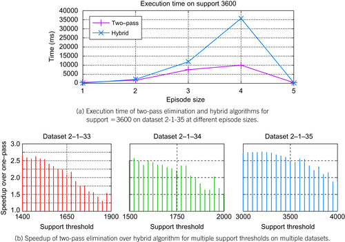 |
| Figure 15.9
Execution time and speedup comparison of the hybrid algorithm versus the two-pass elimination algorithm.
|
We also use
CUDA Visual Profiler
to analyze the execution of the hybrid algorithm and
PreElim
algorithm to give a quantitative measurement of how
PreElim
outperforms the hybrid algorithm on the GPU. We have analyzed various GPU performance factors, such as GPU occupancy, coalesced global memory access, shared memory bank conflict, divergent branching, and local memory loads and
stores. We find the last two factors are primarily attributed to the performance difference between the hybrid algorithm and
PreElim
(see
Figure 15.10
). The hybrid algorithm requires 17 registers and 80 bytes of local memory for each counting thread, whereas
PreElim
algorithm only requires 13 registers and no local memory. Because local memory is used as a supplement for registers and mapped onto global memory space, it is accessed very frequently and has the same high memory latency as global memory. In segment (a) of
Figure 15.10
, the total amount of local memory access of both the two-pass elimination algorithm and the hybrid algorithm comes from the hybrid algorithm. Because the
PreElim
algorithm eliminates most of the nonsupported episodes and requires no local memory access, the local memory access of the two-pass approach is much less than the one-pass approach when the size of the episode increases. At the size of four, the
PreElim
algorithm eliminates all episode candidates; thus, there is no execution for the hybrid algorithm and no local memory access, resulting in a large performance gain for the two-pass elimination algorithm over the hybrid algorithm. As shown in segment (b) of
Figure 15.10
, the amount of divergent branching also affects the GPU performance difference between the two-pass elimination algorithm and the hybrid algorithm.
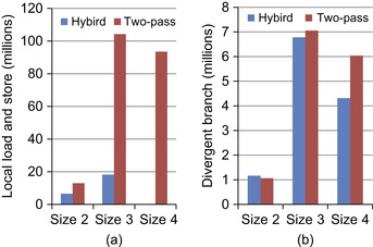 |
| Figure 15.10
Comparison between the hybrid algorithm and two-pass elimination algorithm for support threshold 1650 on dataset
2-1-33
. (a) Total number of loads and stores of local memory. (b) Total number of divergent branches.
|
We have presented a powerful and nontrivial framework for conducting frequent episode mining on GPUs and shown its capabilities for mining neuronal circuits in spike train datasets. For the first time, neuroscientists can enjoy the benefits of data mining algorithms without needing access to costly and specialized clusters of workstations. Our supplementary website (http://neural-code.cs.vt.edu/gpgpu
) provides auxiliary plots and videos demonstrating how we can track evolving cultures to reveal the progression of neural development in real time.
Our future work is in four areas. First, our experiences with the neuroscience application have opened up the interesting topic of mapping finite state machine algorithms onto the GPU. A general framework to map any finite state machine algorithm for counting will be extremely powerful not just for neuroscience, but for many other areas such as (massive) sequence analysis in bioinformatics and linguistics. Second, the development of the hybrid algorithm highlights the importance of developing new programming abstractions specifically geared toward data mining on GPUs. Third, we found that the two-pass approach performs significantly better than running the complex counting algorithm over the entire input. The first pass generates an upper bound that helps reduce the input size for the complex second pass, speeding up the entire process. We seek to develop tighter bounds that incorporate more domain-specific information about neuronal firing rates and connectivities. Finally, we wish to integrate more aspects of the application context into our algorithmic pipeline, such as candidate generation, streaming analysis, and rapid “fast-forward” and “slow-play” facilities for visualizing the development of neuronal circuits.
[1]
S. Adee,
Mastering the brain-computer interface
,
IEEE Spectrum
(2008
)
;
Available from:
http://spectrum.ieee.org/biomedical/devices/mastering-the-braincomputer-interface
.
[2]
M. Harris, S. Sengupta, J.D. Owens,
GPU Gems 3
. (2007
)
Addison Wesley, Pearson Education Inc.
,
Upper Saddle River
;
(Chapter 39)
.
[3]
P. Hingston,
Using finite state automata for sequence mining
,
Aust. Comput. Sci. Commun.
24
(1
) (2002
)
105
–
110
.
[4]
K.E. Iverson,
A Programming Language
. (1962
)
John Wiley & Sons, Inc.
,
New York
.
[5]
S. Laxman, P. Sastry, K. Unnikrishnan,
A fast algorithm for finding frequent episodes in event streams
,
In:
Proceedings of the 13th ACM SIGKDD International Conference on Knowledge Discovery and Data Mining (KDD 2007), San Jose, CA
(August 2007
), pp.
410
–
419
.
[6]
D. Patnaik, P. Sastry, K. Unnikrishnan,
Inferring neuronal network connectivity from spike data: a temporal data mining approach
,
Sci. Program.
16
(1
) (2008
)
49
–
77
.
[7]
S. Sengupta, M. Harris, Y. Zhang, J.D. Owens,
Scan primitives for GPU computing
,
In:
Graphics Hardware
(2007
)
ACM
,
New York
, pp.
97
–
106
.
[8]
D.A. Wagenaar, J. Pine, S.M. Potter,
An extremely rich repertoire of bursting patterns during the development of cortical cultures
,
BMC Neurosci.
(2006
)
10.1186/1471-2202-7-11
.
..................Content has been hidden....................
You can't read the all page of ebook, please click here login for view all page.