
Chapter 22. GPU-Accelerated Ant Colony Optimization
Robin M. Weiss
In this chapter we discuss how GPGPU computing can be used to accelerate ant colony optimization (ACO) algorithms. To this end, we present the AntMinerGPU algorithm, a GPU-based implementation of the AntMiner+ algorithm for rule-based classification. Although AntMinerGPU is a special-purpose ACO algorithm, the general implementation strategy presented here is applicable to other ACO systems, swarm intelligence algorithms, and other algorithms that exhibit a similar execution pattern.
22.1. Introduction, Problem Statement, and Context
In the past decade, the field of swarm intelligence has become a hot topic in the areas of computer science, collective intelligence, and robotics. ACO is a general term used to describe the subset of swarm intelligence algorithms that are inspired by the behaviors exhibited by colonies of real ants in nature. Current literature has shown that ACO algorithms are viable methods for tackling a wide range of hard optimization problems including the traveling salesman, quadratic assignment, and network routing problems
[1]
[2]
and
[3]
.
In nature, ants are simple organisms. Individually, each has very limited perceptual capabilities and intelligence. However, ants are social insects, and it has been observed that groups of ants can exhibit highly intelligent collective behaviors that surpass the capabilities of any given individual. It is these emergent behaviors of ant colonies that ACO algorithms reproduce with colonies of virtual “ant agents” and use for solving computational problems.
In general, ACO algorithms are characterized by a repeated process of probabilistic solution generation, evaluation, and reinforcement. Over time, the solutions generated by ant agents converge to a (near) optimal solution. By generating a larger number of solutions each iteration (which requires a similarly larger population of ant agents), a more complete exploration of solution space can be achieved and thus better solutions can be found in less time. However, the population of ant agents in sequential ACO algorithms is a large factor in overall running time and therefore makes very large ant populations infeasible.
Because ant colonies, both real and virtual, are a type of distributed and self-organizing system, there is a large amount of implicit parallelism. In this chapter we investigate how the GPGPU computing model can take advantage of this parallelism to achieve large populations of ant agents while also reducing overall running time. It is our hope to show that with GPU-based implementations, ACO
algorithms will be seen as competitive with traditional methods for a range of problems. As a case study, we present the GPU-based AntMinerGPU algorithm, an ACO algorithm for rule-based classification, and show how the GPGPU computing model can be leveraged to improve overall performance.
22.2. Core Method
Perhaps the most well-explored feature of ant systems is their ability to locate optimal paths through an environment. This phenomenon forms the basis of the standard ACO metaheuristic. The path-finding ability of ant colonies can be extended to solve problems from a wide range of domains so long as the solution space of the target problem can be expressed as a graph where paths represent solutions. The reader is referred to
[1]
and
[2]
and
[3]
for examples of how various problems can be represented as such.
In ACO, virtual ant agents make explorations of the solution space of a target problem in an attempt to locate the optimal solution. A solution is defined by a path traveled by an ant agent through a graph-based representation of solution space called the “construction graph.” After each solution construction phase, candidate solutions are evaluated with respect to a quantitative fitness function. The path that describes the “best” solution (maximizes the fitness function) is reinforced with “pheromone,” which attracts ant agents in subsequent iterations to a similar path. Over time and with the introduction of random variations in the movements of ant agents, the repeated explorations of solution space often leads to a convergence of the swarm as a whole to the optimal solution. This generalized control flow of ACO algorithms is depicted in
Figure 22.1
.
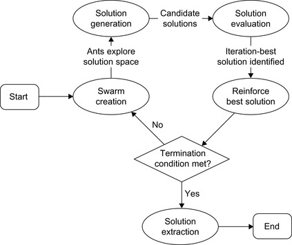 |
| Figure 22.1
The basic scheme of an ACO swarm.
|
22.3.1. Ant Colony Optimization and GPU Computing
The three main phases of ACO algorithms are shown in the high-level pseudo code for ACO given in
Figure 22.2
and further described in the context of AntMinerGPU in the following subsections.
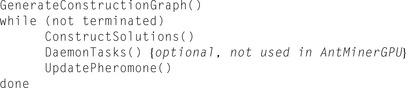 |
| Figure 22.2
High-level pseudo-code overview of the general ACO approach.
|
It is our hypothesis that with a larger population of ant agents than suggested by current literature, higher-quality solutions will be found in less time because more candidate solutions are generated each iteration. However, achieving large populations of ant agents can present a problem with respect to running time. Because each ant is a completely independent agent and requires its own memory and control logic, a sequential implementation forces ants to “take turns” on the processor, each generating a candidate solution one after the next. This is a sub-optimal implementation strategy for ACO algorithms because overall running time will grow directly with the number of ant agents in the system.
With a GPU-based parallel implementation, the computational complexity of ACO can be greatly reduced and can thus allow for efficient execution with very large ant populations. Furthermore, a parallelized implementation in which each ant is allocated its own control thread allows the virtual ant colony to achieve the asynchronous nature of the real ant colonies on which the model is based.
22.3.2. AntMinerGPU Overview
The AntMinerGPU algorithm is an extension of the MAX-MIN Ant System
[8]
and the AntMiner+ algorithm
[6]
. The creators of the original AntMiner algorithm show how the solution space of the rule-based classification problem can be conceived of as a graph and in doing so prove that the ACO technique can be applied
[5]
.
AntMiner+ is the fourth version of the AntMiner algorithm and has been shown to produce higher-quality results and offers a less complex implementation than previous versions
[6]
. For these reasons, AntMiner+ is the version adopted here for GPU-based implementation. The AntMinerGPU algorithm extends AntMiner+ by offloading its implicitly parallel steps to a GPU device. Most notably, we use the multithreading capabilities of the GPU to allocate each ant agent its own thread. In this way, the overall running time of the algorithm is much less affected by the population of ant agents, and therefore, much larger populations can be used.
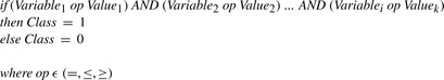
The input to AntMinerGPU is a training dataset where the class of each data point is known. From this, AntMinerGPU iteratively builds up a set of classification rules that can be used to predict the class of new data points. The implementation presented here is concerned with only binary classification (i.e., data points are a member of one of two possible classes). Therefore, rules generated by
AntMinerGPU always attempt to identify the predictive characteristics of data points of class 1, using an explicit “else” statement as the final rule to indicate that any data point not covered by a rule must be of class 0.
Figure 22.3
shows the general form of rules produced by AntMinerGPU.
 |
| Figure 22.3
The general form of classification rules generated by AntMinerGPU.
|
The basic task of ants in AntMinerGPU is to probabilistically select a subset of terms (Variable
i
op Value
k
) where
op
∈ {=, ≤, ≥} from the set of all possible terms (as given by the data being classified) such that when conjoined with the logical AND operator, classification rules that maximize confidence and coverage are produced. The reader is referred to
[9]
for a detailed explanation of rule-based classification and the metrics of confidence and coverage that are used as the quantitative evaluation of solution quality in our algorithm.
The Construction Graph
The AntMinerGPU algorithm uses a directed acyclic graph (DAG) as the representation of solution space. The construction graph,
Gc
(V
,
E
), is generated in such a way that the vertices represent the set of all possible solution components and the existence of some edge
E
ij
represents the ability to select solution component
j
after having selected
i
. With this configuration, a path through
Gc
can be taken as a solution to the target problem, and good solutions can be found by exploiting the collectively intelligent behaviors of ant colonies that allow them to find optimal paths through an environment.
In the case of rule-based classification, the construction graph is generated in such a way that it captures the dimensionality of the feature space of the data to be classified. That is, the construction graph is created by generating one node group for each variable in the training dataset. These node groups are shown as vertical rectangles in
Figure 22.4
. Each group contains nodes representing all possible values that the respective variable may possess.
 |
| Figure 22.4
The general form of the construction graph for AntMinerGPU.
|
Nominal variables are represented by one node group, containing a node for each value the variable may possess, as well as an additional node representing “does not matter.” This “dummy” node can be selected by the ants and signifies that the variable has no bearing on the class that is predicted by the rule. An ant visiting vertex
k
in the group representing nominal variable
i
will add the term (Variable
i
=
Value
k
) to its candidate rule.
The AntMinerGPU algorithm also allows for ordinal variables to be used in the data mining process. For this type of variable, we allow for the selection of terms that can specify a range of values. That is, we allow for terms such as (Variable
i
>=
Value
k
) and (Variable
i
<=
Value
l
). To realize this, ordinal variables are represented by two node groups that represent a lower and upper bound that can be placed on the given variable in candidate classification rules.
V
2 in
Figure 22.4
is an example of this structure.
The movements of ants through the construction graph are restricted by requiring that each variable appear at most once in the final classification rule. This is accomplished by using directed edges in
the construction graph. In the case of nodes representing ordinal variables, the choice of paths is also restricted such that rules that lead to logically unsatisfiable conditions cannot be produced. Specifically, we wish to avoid the situation where a rule specifies (Variable
i
<=
x
)
AND
(Variable
i
>=
y
) where
y
>
x
. To prevent this, we simply remove edges from the construction graph that would allow for this type of path (note that node
n
2, 2
does not connect to node
n
2, 1
).
Solution Construction
In the solution construction phase, a set of
m
ant agents generates candidate classification rules from a finite set of terms (represented by the vertices of
GC
). Solution construction for each ant begins with an empty partial classification rule,
R
p
= Ø. At each construction step,
R
p
is extended by adding an available term to the partial classification rule. This is achieved as ant agents repeatedly move from some node
i
to some node
j
in the construction graph, appending the term represented by
j
to
R
p
, and continuing in this fashion until reaching the end node. The choice of term to add to
R
p
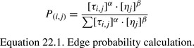
from the set of feasible terms is a probabilistic choice with the probability of selecting term
j
after having selected term
i
given by:
where τ
i,j
is the pheromone associated with edge
E
i,j
, and
η
is the heuristic value of term
j
(α
and
β
being parameters that weight the relative influence of
τ
and
η
). As mentioned, pheromone levels reflect the quality of classification rules produced when other ants traversed the edge, and these pheromones are used to attract ants toward potentially rich areas in the construction graph. The heuristic value
of
j
(η
j
) indicates the importance of node
j
in final solutions. This value is supplied by a problem-dependent function and is derived from a priori knowledge of the problem. The reader is referred to
[6]
for a description of the heuristic value used by the AntMiner class of algorithms.
 |
Pheromone Updating
An ant will select a term to add to its candidate classification rule with a probability that is proportional to the amount of pheromone on the edge leading to it. The objective of pheromone updating is to increase the pheromone levels on paths associated with good solutions (by reinforcement) and to decrease pheromone levels on paths associated with bad solutions (by evaporation). Reinforcing the pheromone levels on edges that comprise “good” solutions attracts ants in later iterations to similar areas of solution space (which are likely to contain other good, if not better, solutions). Evaporation is the process whereby pheromone levels on all graph edges are diminished over time. This allows for trails that were reinforced earlier in the exploration phase, and that may represent suboptimal solutions, to be slowly “forgotten.”
The MAX-MIN Ant System on which AntMinerGPU is based specifies a few requirements for pheromone levels. Before the first exploration of the construction graph by ant agents, all edges are initialized with a pheromone level equal to the parameter
τ
max
. This allows for a more complete exploration of solution space in the early iterations of the algorithm because all edges appear equally attractive with respect to pheromone level.
Pheromone updating is achieved in two phases, evaporation and reinforcement. First, pheromone evaporation is applied to all edges in the construction graph. In this phase, all pheromone levels are multiplied by an evaporation factor (ϱ
) that normally lies in the range between 0.8 and 0.99. The pheromone levels on all edges are bounded to a minimum value (τ
min
) such that edges are prevented from having such a small amount of pheromone on them that they become unexplored altogether.
The process of pheromone reinforcement occurs after evaporation. This phase begins by evaluating the quality of each ant agent's candidate solution with respect to some quantitative fitness function. The MAX-MIN Ant System indicates that only the path representing the iteration-best solution be reinforced with an amount of pheromone proportional to the quality of that solution
[8]
. To realize this, an amount of pheromone is added to all edges of the iteration-best solution equal to the quantitative measure of quality of that solution. The maximum amount of pheromone on an any given edge is bounded by the parameter
τ
max
.
22.3.3. Operational Overview and Implementation Details
The basic operation of the AntMinerGPU algorithm is as follows. At the start of every iteration, ants begin in the start node and walk through the construction graph until reaching the end node. As an ant walks, it makes a probabilistic choice of which edge to traverse based on the amount of pheromone on each available edge, and the heuristic value of the node to which each available edge connects. An ant records the nodes it visits, with each node representing a logical term that is added to the ant's candidate classification rule. Once all ants in a generation reach the end node, each ant's rule is evaluated, and the rule with the best quality is reinforced with pheromone. This process repeats until there is no improvement of the global-best rule for some predefined number of iterations. Then, the global-best rule is outputted, and training data points that are “covered” by that rule are removed from the training dataset. This whole process is then repeated until some minimum percentage of training data points remain. This process is given in pseudo code in
Figure 22.5
.
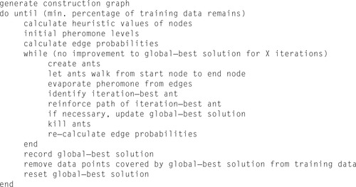 |
| Figure 22.5
Pseudo-code overview of AntMinerGPU.
|
The overall operation of AntMinerGPU is broken down into eight GPU kernel functions. The control flow of AntMinerGPU is diagrammed in
Figure 22.6
. A description of each kernel function and implementation considerations for each follow this diagram.
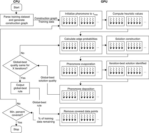 |
| Figure 22.6
The CPU-GPU control flow of AntMinerGPU.
|
Data Structures and General Implementation Considerations
To capture the structure of the construction graph, we implement two structs,
Node
and
Link
. The output of the host-side initialization code is two arrays,
d_nodes
and
d_links
, each a 1-D array containing all
Node
and
Link
structs generated to represent the construction graph for the input dataset.
Node
structs keep track of which edges emanate from each node in order to allow ants to identify which edges are available to them during each stage of solution construction. The
Node
struct contains two
int
values, allowing a
Node
to be read as a single 64-bit chunk. This also alleviates alignment issues as
Node
structs can be neatly packed in memory and accesses can be coalesced.
The important information pertaining to edges (pheromone level, heuristic value of terminal node, and probability of traversal) are stored as
float
values in three separate arrays (d_pheromone
,
d_heuristic
, and
d_probability
). Keeping these values separate allows kernels that may need some combination of them to fetch them individually. Additionally, separating this data as such allows
Link
structs to only contain 4
int
values, allowing them to be aligned neatly in memory. Because there are a number of kernel functions that operate over all links, the
d_pheromone
,
d_heuristic
, and
d_probability
arrays are padded so that their sizes are a multiple of 512 elements. In this way, we can avoid the overhead of checking to see if threads are working within the bounds of the array, and a number of threads equal to the number of links in the padded array can always be safely invoked.
In addition to reading in training data and generating the corresponding construction graph, host-side code also generates an array of the training data itself because this will be needed by the
evaluateTours
and
calculateHeuristic
kernels to compute the quality of candidate solutions and heuristic values of nodes, respectively. Because training data is static, we are able to leverage the performance benefits of caching by binding the training data to a 1-D texture and accessing the data through texture fetch calls. The use of texture caching will be discussed in the following subsections in the context of particular kernel functions.
Pheromone Initialization
This very simple kernel function initializes the pheromone level on all edges in the construction graph to the value supplied by the parameter
tMax
. The
initializePheromones
kernel is passed a pointer to the padded array of pheromone levels,
d_pheromone
, and the parameter
tMax
. Because adjacent
threads store
tMax
to adjacent memory locations, very strong memory coalescing is achieved by this kernel.
__global__ void initializePheromones(float* d_pheromone, float tMax){
int linkID = blockIdx.x * blockDim.x + threadIdx.x;
d_pheromone[linkID] = tMax;
}
Heuristic Value Computation
The heuristic value of a node in the construction graph attempts to capture the importance of that node's value for its variable in classification rules. The heuristic value of a given node is given in
Equation 22.2
. We use the notation |
condition
| to refer to the number of elements in the set of all data points that satisfy
condition
.
 |
calculateHeuristic
is invoked with a number of threads equal to the size of
d_links
arranged in a 1-D grid of 1-D blocks. A thread identifies which link it is responsible for based on its position in the grid. Each thread then iterates over the training data in
d_translatedData
and calculates the heuristic value of the node to which its edge connects to, recording this value in the
d_heuristic
array in the location of the link it is working with.
Edge Probabilities
As detailed earlier in this chapter, the solution-generation process carried out by ant agents is probabilistic. That is, when located on a given node, an ant will elect to traverse a connected edge with some probability as given by
Eq. 22.1
. The task of the
calculateProbabilities
kernel is to precompute edge probabilities. This requires computing the product of the amount of pheromone on an edge and the heuristic value of the node to which the edge connects, divided by the sum of this value computed for all edges emanating from the source node.
The abstraction we make in this kernel is between nodes and blocks. Each node in the construction graph is allocated a block of threads where each thread calculates the probability for an edge emanating from its block's node.
The
calculateProbabilities
kernel is actually quite simple. Each thread identifies which node it is working with based on its block's index in the grid. Then, based on its index within the block, each thread calculates the product of the amount of pheromone and heuristic value associated with its link, retrieving these values from the
d_pheromone
and
d_heuristic
arrays, respectively. The resultant value is then stored in a shared memory array. Once all threads calculate this value for their respective
link, each thread sums these values from shared memory, storing the result in a register. All threads then divide the value it calculated for its link by the sum, storing the result in the
d_probability
array located in global memory. Abbreviated source code for the
calculateProbabilities
kernel is offered below.
extern __shared__ float choices[];
Node n = d_nodes[blockIdx.x];
int idx = threadIdx.x;
if (idx < n.numLinks){
choices[idx] = __powf(d_pheromone[n.firstLink + idx],alpha) * __powf(d_heuristic[n.firstLink + idx], beta);
__syncthreads();
float sum = 0.0f;
for (int i = 0; i < n.numLinks; i++){
sum += choices[i];
}
d_probability[n.firstLink + idx] = choices[idx] / sum;
}
It should be noted that the
calculateProbabilities
kernel is usually invoked with a relatively small number of threads per block. Thus, the occupancy of the
calculateProbabilities
kernel is usually small. However, this abstraction of graph structure to grid organization is the most natural and has been selected here.
Solution Generation
Exploration of the construction graph by the population of ant agents is carried out by the
runGeneration
kernel. The
runGeneration
kernel illustrates one of the most challenging aspects of ACO for GPGPU computing, namely, the probabilistic path selection process. Because each ant may take a different path through the construction graph and because these paths are impossible to predict, little can be done to ensure orderly memory transactions and concurrency.
The
runGeneration
kernel is passed a pointer to
d_nodes
,
d_probability
, and an array of random number seeds,
d_random
. It is invoked with a number of threads equal to the number of ants in the system, arranged into a 1-D grid of 1-D blocks. Each thread calculates which ant it represents based on its position in the grid.
All threads enter a loop for a number of iterations equal to the number of node groups in the construction graph. In each pass of the loop, a new link is added to each ant's tour. Threads generate a new random number based on their seeds and a simple Park-Miller pseudorandom number generator. This pseudorandom number is then used in a roulette-wheel selection process to probabilistically select an edge to traverse. When an ant selects an edge to traverse, it adds the index of the edge it traverses to an array in global memory that records the paths of all ants in the generation.
The
evaporizePheromone
kernel is very similar to the
initializePheromone
kernel in that a simple function is being applied to all values in the
d_pheromone
array. In this case, the kernel must read in each value from
d_pheromone
, multiply it by a supplied parameter, and store the result back to
d_pheromone
. As in
initializePheromone
, adjacent threads in
evaporizePheromone
read and write values to adjacent memory locations and, therefore, strong memory coalescing is achieved in this kernel as well. The source code for this kernel is provided here. It should be noted that the array
d_pLevels
contains the values of parameters
<tau>_min
and
<tau>_max
in locations 0 and 1, respectively.
__global__ void evaporizePheromone(float evaporize,float* d_pLevels, float* d_pheromone){
int linkID = blockIdx.x * blockDim.x + threadIdx.x;
float p = d_pheromone[linkID] *= evaporize;
if (p < d_pLevels[0]) d_pheromone{
[linkID] = d_pLevels[0];
}
}
Solution Evaluation
Solution evaluation is the most costly portion of the AntMinerGPU algorithm. This phase necessitates comparing each ant's tour to the entirety of the training dataset to identify how many training data points each ant's tour accurately describes. Thus, this kernel requires a very large amount of memory transactions because each training data point must be analyzed.
The implementation strategy we have adopted here is depicted in
Figure 22.7
. The abstraction we make is between ants and blocks. That is, the threads of one block are collectively responsible for evaluating the respective ant's tour against all training data points. Each block contains a number of helper threads equal to the number of data points,
m
, in the training dataset (or the maximum number of threads per block if
m
is greater than this value).
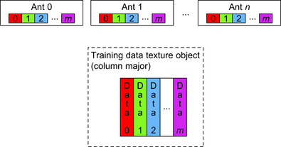 |
| Figure 22.7
Thread allocation abstraction for solution-evaluation kernel.
|
The heart of the
evaluateTours
kernel is a for-loop that iterates over each term in the block's candidate classification rule. For each term, the helper thread must determine whether its training data point is accurately described by its ant's candidate classification rule. By storing the training dataset in column major form, consecutive helper threads access consecutive memory locations. Because of the spatial locality exhibited by this access pattern, we have found that texture caching provides performance benefits. In fact, testing reveals an average texture cache hit rate of ∼40% in the
evaluateTours
kernel and running time of this kernel is reduced by nearly 25%.
Recall that the goal of the
evaluateTours
kernel is to determine how many training data points are described by each ant's rule. In our implementation strategy, we use an atomic add operation on a shared memory location to accumulate this value across all helper threads. That is, once each helper thread evaluates whether or not the ant's tour accurately predicts its designated data point, the helper thread will increment the shared memory accumulator atomically. Although this method implies some degree of serialization will occur, we have found the performance impact to be small compared with other approaches.
After the result of each helper thread is recorded, a thread will select a new data point to consider if
m
is greater than the maximum number of threads allowed per block. Here is abbreviated source code for this kernel function.
int antID = blockIdx.x;
int idx = threadIdx.x;
// shared data structures
int* s_tour;
// the tour of the ant this block is responsible for
int* s_covered;
// how many data points are covered by the solution
int* s_correct;
// how many data points are accurately described by the solution
int* s_graphVarType;
// what type of term (==, <=, or >=) each term is
int* s_graphVarID;
// what variable in the training data each term pertains to
…
__syncthreads();
int dataID = idx;
while (dataID < dataCount){
int test = 0;
if (d_classOf[dataID] != −1){
for (int j = 0; j < graphVarCount; j++){
int tourValue = s_tour[j];
int varType = s_graphVarType[j];
int dataValue = tex1Dfetch(translatedDataTEX, s_graphVarID[j] * dataCount + dataID);
// Test tourValue against dataValue
// if tourValue == dataValue, test++
}
if (test == graphVarCount){
atomicAdd(s_covered, 1);
if (d_classOf[dataID] == 1){
atomicAdd(s_correct, 1);
}
}
}
}
__syncthreads();
if (idx == 0){
// Implement fitness function, storing result in d_quality[antID]
}
Pheromone Deposition
AntMinerGPU deposits pheromone only on the best path of all ants in a generation. Therefore, the quality of each ant's path must be considered to determine which ant generated the “best” solution. This is accomplished by a kernel function that copies the quality of each ant's tour into shared memory and then applies a reduction to determine which ant generated the best quality tour. Once the iteration-best ant has been identified, a number of threads equal to the number of node groups in the construction graph adds an amount of pheromone to the links in the iteration-best ant's tour.
Remove Covered Data Points
Once a predefined number of iterations pass with no improvement to the global-best solution, the global-best rule is outputted, and data points described by that rule must be removed from the training dataset. To accomplish this, we invoke the kernel
flagCoveredCases
with a number of threads equal to the number of training data points. Each thread checks to see if the global-best solution describes the data point it is responsible for. If so, the class of that data point is set to −1, indicating that the data point has been covered. The internal workings of this kernel are very similar to that of the
evaluateTours
kernel.
22.4. Final Evaluation
To evaluate the performance benefits of our GPU-based implementation of AntMiner+, we ran AntMinerGPU on two simple datasets to compare the accuracy and running time against that given by a CPU-based implementation of AntMinerGPU. The datasets used were the Wisconsin Breast Cancer (WBC) and Tic-Tac-Toe (TTT), both of which were downloaded from the UCI Machine Learning Repository
[7]
.
To split the datasets into training and testing sets, the order of data points in each set was first randomized, and then the first two-thirds of the data points were taken as training data with the remaining data points used as testing data. Because AntMinerGPU is a stochastic algorithm, results can vary from run to run. For this reason, the metrics we report are average values derived from 15 independent runs on three different random splits of the given dataset. The same random splits were used on both CPU and GPU implementations. Results presented later in this chapter were gathered on a desktop computer system with a 2.4GHz Intel Core 2 Quad processor and 3GB of DDR3 memory. The GPU device used was an NVIDIA Tesla C1060.
To determine the effect of ant population, we ran AntMinerGPU with a range of populations, plotting this variable against accuracy of rules generated for the WBC dataset (in
Figure 22.8a
) and the TTT dataset (in
Figure 22.9a
). We also plotted the effect of ant population on running time in
Figure 22.8
and
Figure 22.9
for the WBC and TTT datasets, respectively. Also included in these plots are results obtained from a CPU-based implementation of AntMinerGPU for comparison.
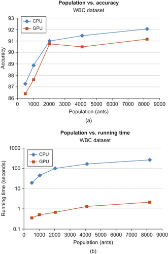 |
| Figure 22.8
(a) Comparison of the effect of population size on accuracy of classification rules for the WBC dataset for both CPU- and GPU-based implementations. (b) Comparison of the effect of population size on running time of the AntMinerGPU algorithm for the WBC dataset for both CPU- and GPU-based implementations.
|
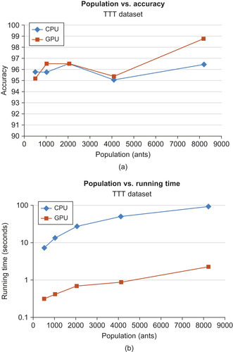 |
| Figure 22.9
(a) Comparison of the effect of population size on accuracy of classification rules for the TTT dataset for both CPU- and GPU-based implementations. (b) Comparison of the effect of population size on running time of the AntMinerGPU algorithm for the TTT dataset for both CPU- and GPU-based implementations.
|
We found that in general, the accuracy of GPU- and CPU-based implementations were very similar. In terms of running time, we found that the GPU-based implementation is up to 100x faster than the simple CPU-based implementation for large populations of ants.
Perhaps the most promising area of exploration for GPU-based ACO algorithms is in multi-colony implementations on multiple GPUs. ACO algorithms are notoriously dependent on parameter settings, and therefore, running multiple ACO algorithms with varying parameters on multiple GPUs could
allow for the optimal settings to be found for a given problem. Additionally, because ACO algorithms are stochastic, some runs are better than others. To take advantage of this, it is possible that multiple instances of AntMinerGPU may be run concurrently, perhaps on a multi-GPU computer system, and the instance with the best performance be taken as the final solution.
Another area for improvement of AntMinerGPU is in the boundary placed on it by limited GPU memory. In order to store much larger training datasets in GPU memory, we propose that a pre-processing step could be used to translate the values of the input dataset into
short int
values. This step would generate a lookup table that would be stored in CPU memory and could be used to translate between these short integer “value codes” and the actual values that they represent. By translating input data to
short int
form, we can load twice the amount of data onto the GPU as compared with using
int
or
float
data types. This step would, of course, introduce more running time because preprocessing and postprocessing are required, but would allow for larger datasets to be classified.
Acknowledgments
Support for this research was provided by NSF grants for Mathematics and Geophysics (CMG) and an equipment grant from CRI awarded to the LCSE of the University of Minnesota. I would also like to thank my advisors David Yuen, Witold Dzwinel, and Marcin Kurdziel for their ideas and advice throughout the development process of this software.
References
[1]
M. Dorigo, G.D. Caro,
Ant algorithms for discrete optimization
,
Artif. Life
5
(1999
)
137
–
172
.
[2]
M. Dorigo, G. Di Caro,
The ant colony optimization meta-heuristic
,
In: (Editors: D. Corne, M. Dorigo, F. Glover)
New Ideas in Optimization
(1999
)
McGraw-Hill
,
Maidenhead, UK, England
, pp.
11
–
32
.
[3]
M. Dorigo, T. Stützle,
Ant colony optimization
. (2004
)
MIT Press
,
Cambridge, MA
.
[4]
R.S. Parpinelli, H.S. Lopes, A.A. Freitas,
An ant colony based system for data mining: application to medical data
,
In: (Editors: L. Spector, E. Goodman,
et al.
)
Proceedings of the Genetic and Evolutionary Computation Conference, Morgan Kaufmann Publishers, San Francisco, CA, San Francisco, CA, July 7–11
(2001
), pp.
791
–
797
.
[5]
B. Liu, H.A. Abbass, B. McKay,
Classification rule discovery with ant colony optimization
,
IEEE Comput. Intell. Bull.
3
(1
) (2004
)
31
–
35
.
[6]
D. Martens, M.D. Backer, R. Haesen, B. Baesens, T. Holvoet,
Ants constructing rule-based classifiers
,
Stud. Comput. Intell.
34
(2006
)
21
–
43
.
[7]
UCI Machine Learning Repository, University of California, School of Information and Computer Science, Irvine, CA
http://archive.ics.uci.edu/ml/
(2010
)
;
(accessed 20.03.10)
.
[8]
T. Stutzle, H. Hoos, Improving the ant-system: a detailed report on the max-min ant system (Technical Report), FG Intellektik, FB Informatik, TU Darmstadt, Germany, 1996.
[9]
P. Tan, M. Steinbach, V. Kumar,
Introduction to data mining
.
first ed.
(2006
)
Pearson
,
Boston, MA
;
pp. 207–223
.
..................Content has been hidden....................
You can't read the all page of ebook, please click here login for view all page.