
Chapter 25. Lattice Boltzmann Lighting Models
Robert Geist and James Westall
In this chapter, we present a GPU-based implementation of a photon transport model that is particularly effective in global illumination of participating media, including atmospheric geometry such as clouds, smoke, and haze, as well as densely placed translucent surfaces. The model provides the “perfect” GPU application in the sense that the kernel code can be structured to minimize control flow divergence and yet avoid all memory bank conflicts and uncoalesced accesses to global memory. Thus, the speedups over single-core CPU execution are dramatic. Example applications include clouds, plants, and plastics.
25.1. Introduction, Problem Statement, and Context
Quickly and accurately capturing the the process of light scattering in a volume filled with a participating medium remains a challenging problem, but often it is one that must be solved to achieve photo-realistic rendering. The scattering process can be adequately described by the standard volume radiative transfer equation
 where
where
 is a position in space,
 is a spherical direction,
 is the phase function,
σ
s
is the scattering coefficient,
σ
a
is the absorption coefficient,
σ
t
=
σ
s
+
σ
a
is the extinction coefficient, and
is the phase function,
σ
s
is the scattering coefficient,
σ
a
is the absorption coefficient,
σ
t
=
σ
s
+
σ
a
is the extinction coefficient, and
 is any emissive field within the volume
[1]
. This simply says that the change in radiance along any path includes the loss due to absorption and out-scattering (coefficient −
σ
t
) and the gain due to in-scattering from other paths (coefficient
σ
s
).
is any emissive field within the volume
[1]
. This simply says that the change in radiance along any path includes the loss due to absorption and out-scattering (coefficient −
σ
t
) and the gain due to in-scattering from other paths (coefficient
σ
s
).
(25.1)
Radiative transfer in volumes is a well-studied topic, and many methods for solving
Eq. 25.1
have been suggested. Most are a variation on one of a few central themes. Rushmeier and Torrance
[25]
used a
radiosity
(finite-element) technique to model energy exchange between environmental zones and hence capture isotropic scattering. Their method requires computing form factors between all pairs of volume elements. Bhate and Tokuta
[2]
extended this approach to anisotropic scattering, at the cost of additional form-factor computation.
The most popular approach is undoubtedly the
discrete ordinates method
[3]
in which
Eq. 25.1
is discretized to a spatial lattice with a fixed number of angular directions in which light may propagate.
The need to compute only local lattice point interactions, rather than form factors between all volumes, substantially reduces the computational complexity. Max
[21]
and Languènou
et al
.
[20]
were able to capture anisotropic effects using early variations on this technique. It is well known, however, that this discretization leads to two types of potentially visible errors: (1) light smearing caused by repeated interpolations and (2) spurious beams, called the ray effect. Fattal
[8]
has recently suggested a method that significantly ameliorates both. Successive iteration across six collections of 2-D maps of rays, along which light is propagated, is employed. The 2-D maps are detached from the 3-D lattice, thus allowing a much finer granularity in the angular discretization. Execution time for grids of reasonable size (e.g., 128
3
) is several minutes. Kaplanyan and Dachsbacher
[17]
have recently provided a real-time variation on the discrete ordinates method that is principally aimed at single-bounce, indirect illumination. The method propagates virtual point lights along axial cells by projecting illumination to the walls of an adjacent cell and then constructing a new point light in the adjacent cell that would deliver exactly that effect. It is not immune to either light smearing or the ray effect, and thus the authors restrict its use to low-frequency lighting. The method is extremely fast, largely owing to relatively low-resolution nested grids that are fixed in camera space and give higher resolution close to the viewer.
A third central theme, and that to which our own method may be attached, is the
diffusion approximation
. Stam
[27]
, motivated by earlier work of Kajiya and Von Herzen
[16]
in lighting clouds, observed that a two-term Taylor expansion of diffuse intensity in the directional component only could be substituted into
Eq. 25.1
to ultimately yield a diffusion process that is an accurate approximation for highly scattering (optically thick) media. Jensen
et al
.
[15]
showed that a simple two-term approximation of radiance naturally leads to a diffusion approximation that is appropriate for a highly scattering medium. This was later extended to include thin translucent slabs and multilayered materials
[7]
.
In
[11]
we introduced an approach to solving
Eq. 25.1
based on a Lattice Boltzmann technique and showed how this might be applied to lighting participating media such as clouds, smoke, and haze. In
[12]
we extended this approach to capture diffuse transmission, interobject scattering, and ambient occlusion, such as needed in photo-realistic rendering of dense forest ecosystems. Most recently, we showed that the technique could be parameterized to allow real-time relighting of scenes in response to movement of light sources
[28]
.
As originally described in
[11]
, the technique was effective, but slow. The technique is grid based, and a steady-state solution for a grid of reasonable size (128
3
nodes) originally required more than 30 minutes on a single CPU. Our goal here is to provide the details of a GPU-based implementation that, for this same size grid, will run on a single GPU in 2 seconds. Example lighting tasks will include clouds, plants, and plastics.
25.2. Core Methods
Lattice Boltzmann (LB) methods are a particular class of
cellular automata
(CA), a collection of computational structures that can trace their origin at least back to John Conway's famous
Game of Life
[10]
, which models population changes in a hypothetical society that is geographically located on a rectangular grid. In Conway's game, each grid site follows only local rules, based on nearest-neighbor population, in synchronously updating itself as populated or not, and yet global behavior emerges in
the form of both steady-state colonies and migrating bands of “beings” who can generate new colonies or destroy existing ones.
Arbitrary graphs and sets of rules for local updates can be postulated in a general CA, but those that are most interesting exhibit a global behavior that has some provable characteristic. Lattice Boltzmann methods also employ synchronous, neighbor-only update rules on a discrete grid, but the discrete populations have been replaced by continuous distributions of some quantity of interest. The result is that the provable characteristic is often quite powerful: the system is seen to converge, as lattice spacing and time step approach zero, to a solution of a targeted class of partial differential equations (PDEs).
Lattice Boltzmann methods are thus often regarded as computational alternatives to finite-element methods (FEMs) for solving coupled systems of PDEs. The methods have provided significant successes in modeling fluid flows and associated transport phenomena
[4]
[13]
[26]
[29]
and
[31]
. They provide stability, accuracy, and computational efficiency comparable to finite-element methods, but they realize significant advantages in ease of implementation, parallelization, and an ability to handle interfacial dynamics and complex boundaries.
The principal drawback to the methods, compared with FEMs, is the counterintuitive direction of the derivation they require. Differential equations describing the macroscopic system behavior are derived (emerge) from a postulated computational update (the local rules), rather than the reverse. Thus, a relatively simple computational method must be justified by a derivation that is often fairly intricate.
In the section titled “Derivation of the Diffusion Equation,” we provide the derivation of the parameterized diffusion equation for our lighting model. On one hand, the derivation itself is totally irrelevant to the implementation of the LB lighting technique proposed here, and users of the technique may feel free to skip it entirely. On the other hand, if the processes of interest to the user vary, beyond simple parameter changes, from our basic diffusion process, a new derivation will be required, and it is extremely valuable to have such a sample derivation at hand.
25.3. Algorithms, Implementation, and Evaluation
Lattice Boltzmann methods are grid based, and so, we begin with a standard 3-D lattice, a rectangular collection of points with integer coordinates in 3-D space. A complication of LB methods in three dimensions is that isotropic flow, whether it is water or photon density, requires that all neighboring lattice points of any site (lattice point) be equidistant. A standard approach, owing to d'Humiéres, Lallemand, and Frisch
[6]
, is to use 24 points equidistant from the origin in 4-D space and project onto 3-D. The points are:
 and projection is truncation of the fourth component, which yields 18 directions, that is, the vectors from the origin in 3-D space to each of the projected points. Axial directions then receive double weights. Representation of several phenomena, including energy absorption and energy transmission, is facilitated by adding a direction from each lattice point back to itself, which thus yields 19 directions, the non-corner lattice points of a cube of unit radius.
The key quantity of interest is the per-site photon density. We store this value at each lattice point and then simulate transport by synchronously updating all the values in discrete time steps according to a single update rule. Let
 denote the density at lattice site
 at simulation time
t
that is moving in cube direction
at simulation time
t
that is moving in cube direction
 ,
m
∈ {0, 1, …, 18}. If the lattice spacing is
λ
and the simulation time step is
τ
, then the update (local rule) is:
,
m
∈ {0, 1, …, 18}. If the lattice spacing is
λ
and the simulation time step is
τ
, then the update (local rule) is:
 where Ω
m
denotes row
m
of a 19 × 19 matrix, Ω, that describes scattering, absorption, and (potentially) wavelength shift at each site. If
where Ω
m
denotes row
m
of a 19 × 19 matrix, Ω, that describes scattering, absorption, and (potentially) wavelength shift at each site. If
 denotes total site density, then the derivation in the the section titled “Derivation of the Diffusion Equation” shows that the limiting case of
Eq. 25.2
as
λ
,
τ
→ 0 is the diffusion equation
denotes total site density, then the derivation in the the section titled “Derivation of the Diffusion Equation” shows that the limiting case of
Eq. 25.2
as
λ
,
τ
→ 0 is the diffusion equation
 where the diffusion coefficient
 As noted, this is consistent with previous approaches to modeling multiple photon scattering events
[15]
and
[27]
, which have invariably led to diffusion processes.
As noted, this is consistent with previous approaches to modeling multiple photon scattering events
[15]
and
[27]
, which have invariably led to diffusion processes.
(25.2)
(25.3)
(25.4)
For any Lattice Boltzmann method, the choice of the so-called collision matrix, Ω, is not unique. Standard constraints are conservation of mass,
 , and conservation of momentum,
 , where
 and
and
 represents any site external force. Here, as in
[11]
[12]
[13]
and
[28]
, for the case of isotropic scattering, we specify Ω as follows:
represents any site external force. Here, as in
[11]
[12]
[13]
and
[28]
, for the case of isotropic scattering, we specify Ω as follows:
For row 0:
 For the axial rows,
i
= 1, …, 6:
For the axial rows,
i
= 1, …, 6:
 For the nonaxial rows,
i
= 7, …, 18:
For the nonaxial rows,
i
= 7, …, 18:
 Entry
i
,
j
controls scattering from direction
Entry
i
,
j
controls scattering from direction
 into direction
 , and thus the nondiagonal entries are scaled values of the scattering coefficient for the medium,
σ
s
. Diagonal entries must include out-scattering, −
σ
t
, and, as noted earlier, isotropic flow requires double weights (scale factors) on the axial directions. Directional density
f
0
holds the absorption/emission component. On update, that is, Ω ⋅
f
, fraction
σ
a
from each directional density will be moved into
f
0
. The entries of Ω are then multiplied by
the density of the medium at each lattice sight so that a zero density yields a pass-through in
Eq. 25.2
and a density of 1 yields a full scattering.
, and thus the nondiagonal entries are scaled values of the scattering coefficient for the medium,
σ
s
. Diagonal entries must include out-scattering, −
σ
t
, and, as noted earlier, isotropic flow requires double weights (scale factors) on the axial directions. Directional density
f
0
holds the absorption/emission component. On update, that is, Ω ⋅
f
, fraction
σ
a
from each directional density will be moved into
f
0
. The entries of Ω are then multiplied by
the density of the medium at each lattice sight so that a zero density yields a pass-through in
Eq. 25.2
and a density of 1 yields a full scattering.
(25.5)
(25.6)
(25.7)
Of course, in general, scattering is anisotropic and wavelength dependent. Anisotropic scattering is incorporated by multiplying
σ
s
that appears in entry Ω
i
,
j
by a normalized phase function:
 where
p
i, j
(g
) is a discrete version of the Henyey-Greenstein phase function
[14]
,
where
p
i, j
(g
) is a discrete version of the Henyey-Greenstein phase function
[14]
,
 Here
Here
 is the normalized direction,
 . Parameter
g
∈ [−1, 1] controls scattering direction. Value
g
> 0 provides forward scattering,
g
< 0 provides backward scattering, and
g
= 0 yields isotropic. Mie scattering
[9]
is generally considered preferable, but the significant approximations induced here by a relatively coarse grid render the additional complexity unwarranted. Note that
Eq. 25.8
, which first appeared in
[12]
, differs from the treatment in
[11]
, in that setting
σ
a
= 0 and
g
= 1 yields an effect that is identical to a pass-through.
. Parameter
g
∈ [−1, 1] controls scattering direction. Value
g
> 0 provides forward scattering,
g
< 0 provides backward scattering, and
g
= 0 yields isotropic. Mie scattering
[9]
is generally considered preferable, but the significant approximations induced here by a relatively coarse grid render the additional complexity unwarranted. Note that
Eq. 25.8
, which first appeared in
[12]
, differs from the treatment in
[11]
, in that setting
σ
a
= 0 and
g
= 1 yields an effect that is identical to a pass-through.
(25.8)
(25.9)
If the media in the model are presumed to interact with all light wavelengths in an identical way, then
 can be considered to be the luminance density. In our cloud lighting example of
Section 25.3.2
, this is the case.
can be considered to be the luminance density. In our cloud lighting example of
Section 25.3.2
, this is the case.
Otherwise, as in our other examples, each discrete wavelength to be modeled is characterized by appropriate scattering parameters and phase function. The Lattice Boltzmann model is run once for each parameter set, and the results are combined in a post-processing (ray-tracing) step.
An alternative approach is to implement
 as a vector of per-wavelength densities and run the model one time. This approach can be used to incorporate wavelength shifts during the collision process.
The model is thus completely specified by a choice of
g
,
σ
a
, and
σ
s
, any of which can be wavelength-dependent.
Initial conditions include zero photon density in all directions at all interior nodes in the lattice. For each node in the lattice boundary, directions that have positive dot products with the external light source direction will receive initial photon densities that are proportional to these dot products. These directional photon densities on boundary nodes are fixed for the duration of the execution. Any flow (movement of photon density) into a boundary node is ignored, as is any flow out of a boundary node that goes off lattice.
25.3.1. An OpenCL Implementation
The fundamental update in
Eq. 25.2
must be synchronous. Each lattice site must read 19 values and write 19 values at each time step, but the layout is particularly well suited to GPU architectures in that there is no overlap in sites read or sites written between or among sites. We have implemented kernels for the update in both CUDA and OpenCL for the NVIDIA GTX 480, and we find, after optimizations of both, essentially no speed difference. Thus, in the interest of greater portability, we present the OpenCL solution here.
We use two copies of the directional densities,
 , and ping-pong between them as we advance the time step,
t
. Experience indicates that a final time of
n
×
τ
, where
n
is twice the longest edge dimension of the lattice, will suffice to achieve near-equilibrium values.
, and ping-pong between them as we advance the time step,
t
. Experience indicates that a final time of
n
×
τ
, where
n
is twice the longest edge dimension of the lattice, will suffice to achieve near-equilibrium values.
Both the collision matrix, Ω, and the per-site density of the medium are constant for the duration of the computation. The Ω matrix, which is 19 × 19, easily fits in constant memory, and so we can take advantage of the caching effects there. The medium density is one float per lattice site, which is too large for constant memory, but each lattice site reads only one medium density value per update, and that value can be stored in a register.
In addition to storage for Ω and storage for the per-site medium density, GPU-side storage includes two arrays for the flows:
cl_mem focl[2][WIDTH*HEIGHT*DEPTH*DIRECTIONS];
and a single integer array
dist[WIDTH*HEIGHT*DEPTH*DIRECTIONS];
which holds, for each lattice site and each direction, the flow array index where exiting flow should be placed. The values for
dist[]
can be calculated and stored by the CPU during initialization.
On the CPU side, the entire update, using kernel
mykrn_update
, command queue
mycq
, and lattice dimension
LDIM
is then given by:
void run_updates()
{
int t, from = 0;
cl_event wait[1];
for(t=0;t<FINAL_TIME;t++,from = 1−from){
clSetKernelArg(mykrn_update,0,sizeof(cl_mem),(void *)&focl[from]);
clSetKernelArg(mykrn_update,1,sizeof(cl_mem),(void *)&focl[1-from]);
clEnqueueNDRangeKernel(mycq,mykrn_update,3,0,ws,lws,0,0,&wait[0]);
clWaitForEvents(1,wait);
}
clEnqueueReadBuffer(mycq,focl[from],CL_TRUE,0,LDIM*sizeof(float),&+6;f[0], 0,NULL,NULL);
return;
}
The work size,
ws
, is a three-dimensional integer vector with value (WIDTH, HEIGHT, DEPTH), the dimensions of the the grid. The local work size,
lws
, which specifies threads per scheduled block, is (1, 1, DEPTH), for reasons to be specified shortly.
A naive but conceptually straightforward kernel is then given by
__kernel void update(__global float* from, __global float* to,__global int* dist, __global float* omega, __global float* density)
{
int i = get_global_id(0);
int j = get_global_id(1);
int k = get_global_id(2);
float medium_density, new_flow;
medium_density = density(i,j,k);
for(m=0;m<DIRECTIONS;m++){
new_flow = 0.0f;
for(n=0;n<DIRECTIONS;n++) new_flow += omega(m,n)*from(i,j,k,n);
to[dist(i,j,k,m)] = from(i,j,k,m) + new_flow*medium_density;
}
}
The
from
and
to
arguments hold addresses of the two copies of the flow values. Macros
from(i,j,k,n)
,
dist(i,j,k,m)
, and
omega(m,n)
simply provide convenient indexing into the arrays of the same names, which are necessarily one-dimensional in GPU storage. Both the
from
and
to
arrays hold an extra index, a “sink,” and if the exiting flow from any site in any direction would be off lattice, the value of the
dist(i,j,k,m)
index is this “sink.”
This kernel is attractive in its simplicity, and it offers zero control flow divergence because there are no conditionals. Nevertheless, although the kernel will produce correct results, its performance advantage over a CPU implementation is modest. For the 256 × 128 × 128 array used in the first example of the next section, a CPU implementation running on an Intel i7 X980 3.33 GHz processor required 19.5 minutes. The OpenCL implementation with this kernel required 2.8 minutes. With kernel modifications, the total execution time can be reduced to 6 seconds, of which 1 second is CPU initialization and 5 seconds are GPU execution.
The first important modification is to avoid reloading the values,
from(i,j,k,n)
, from global device memory. Instead, we force storage into registers by declaring 19 local variables,
float f00, f01, …, f18
We then load each directional value once, unroll the interior loop, and use these local variable values instead of
from(i,j,k,n)
.
The second important modification is to rearrange storage to facilitate coalescing of memory requests. Because we have WIDTH × HEIGHT × DEPTH lattice sites, and each of these has 19 DIRECTIONS, it is natural to access linear storage as
from[((((i)*HEIGHT+(j))*DEPTH+(k))*DIRECTIONS+(m))]
but this leads to relatively poor performance. Instead, since DEPTH is usually a large power of 2, we interchange DEPTH and DIRECTIONS so that the DEPTH index varies most rapidly in linear storage:
from[((((i)*HEIGHT+(j))*DIRECTIONS+(m))*DEPTH+(k))]
This rearrangement applies to both copies of the photon density values,
focl[2]
, and the integer
dist[]
array.
The third modification, though least important in terms of performance gained, is probably the most surprising. Performance improves when we add conditionals and extra computation to this kernel! In particular, if we eliminate the
dist[]
array, instead pass only the 19 directions, and calculate the indices for the exiting photon density on the fly, performance improves by a small amount. The conditionals and
the index computations, which are required to avoid indices that would be off lattice, are less expensive than accesses to the global
dist[]
array. Because flow divergence then occurs only between boundary nodes and interior nodes, and we place each DEPTH stripe in a single thread block using local work size (1, 1, DEPTH), the effect of divergence is really minimal.
The final kernel is then given by
#define nindex(i,j,k) (((i)*HEIGHT+(j))*DEPTH+(k))
#define bindex(i,j,k) ((((i)*HEIGHT+(j))*DIRECTIONS*DEPTH)+(k))
#define dindex(i,j,k,m) ((((i)*HEIGHT+(j))*DIRECTIONS+(m))*DEPTH+(k))
#define inbounds(q,r,s) ((q > 0)&&(q < (WIDTH − 1))&&(r > 0)&&(r < (HEIGHT − 1))&&(s > 0)&&(s < (DEPTH − 1)))
__kernel void update(__global float* from,__global float* to,__constant int* direction, __constant float* omega,__global float* density)
{
const int i = get_global_id(0);
const int j = get_global_id(1);
const int k = get_global_id(2);
const int lnindex = nindex(i,j,k);
const int lbindex = bindex(i,j,k);
int m;
float cloud_density, new_flow;
float f00, f01, f02, f03, …, f18;
int outi, outj, outk;
cloud_density = density[lnindex];
f00 = from[lbindex+0*DEPTH];
f01 = from[lbindex+1*DEPTH];
f02 = from[lbindex+2*DEPTH];
f03 = from[lbindex+3*DEPTH];
…
f18 = from[lbindex+18*DEPTH];
for(m=0;m<DIRECTIONS;m++)
outi = i+direction[3*m+0];
outj = j+direction[3*m+1];
outk = k+direction[3*m+2];
if(inbounds(outi,outj,outk))
new_flow = 0.0f;
new_flow += omega(m,0)*f00;
new_flow += omega(m,1)*f01;
new_flow += omega(m,2)*f02;
new_flow += omega(m,3)*f03;
…
new_flow += omega(m,18)*f18;
to[dindex(outi,outj,outk,m)] = from[lbindex+m*DEPTH] + new_flow*cloud_density;
}
}
}
Profiling this kernel shows 100% coalesced global memory reads and writes and an occupancy of 0.5. Transfer from/to global memory is measured at 67 GB/sec., which is a significant portion of the available bandwidth for the GTX 480 as reported by the
oclBandwidthTest
utility, 115 GB/sec. Note that this does not include transfer from (cached) constant memory, which is significantly larger, 718 GB/sec.
On devices of lower compute capability, this kernel can generate a significant number of uncoalesced global memory writes. Nevertheless, with a simple kernel modification we can force these writes to be coalesced as well. Because we use a local work size vector of (1, 1, DEPTH), we can collect DEPTH output values, one for each
outk
, in a local (shared) memory array of size DEPTH, synchronize the threads using a
barrier()
command, and then write the entire DEPTH stripe in order. The final kernel, revised for this lower compute capability, is then:
#define nindex(i,j,k) (((i)*HEIGHT+(j))*DEPTH+(k))
#define bindex(i,j,k) ((((i)*HEIGHT+(j))*DIRECTIONS*DEPTH)+(k))
#define dindex(i,j,k,m) ((((i)*HEIGHT+(j))*DIRECTIONS+(m))*DEPTH+(k))
#define inbounds(q,r,s) ((q > 0)&&(q < (WIDTH − 1))&&(r > 0)&&(r < (HEIGHT − 1))&&(s > 0)&&(s < (DEPTH − 1)))
__kernel void update(__global float* from,__global float* to,__constant int* direction, __constant float* omega,__global float* density)
{
const int i = get_global_id(0);
const int j = get_global_id(1);
const int k = get_global_id(2);
const int lnindex = nindex(i,j,k);
const int lbindex = bindex(i,j,k);
__local float getout[DEPTH];
float cloud_density, new_flow;
float f00, f01, f02, f03, …, f18;
int m, outi, outj, outk;
cloud_density = density[lnindex];
f00 = from[lbindex+0*DEPTH];
f01 = from[lbindex+1*DEPTH];
f02 = from[lbindex+2*DEPTH];
…
f18 = from[lbindex+18*DEPTH];
for(m=0;m<DIRECTIONS;m++){
outk = k+direction[3*m+2];
if(outk>0 && outk<(DEPTH − 1)
new_flow = 0.0f;
new_flow += omega(m,0)*f00;
new_flow += omega(m,1)*f01;
new_flow += omega(m,2)*f02;
…
new_flow += omega(m,18)*f18;
getout[outk] = from[lbindex+m*DEPTH] + new_flow*cloud_density;
}
outi = i+direction[3*m+0];
outj = j+direction[3*m+1];
if(inbounds(outi,outj,k))
to[dindex(outi,outj,outk,m)] = getout[k];
}
}
Testing this modified kernel on a Quadro FX 5600 (compute capability 1.0) shows that it entirely eliminates the uncoalesced writes generated by the original kernel. Execution time performance improves by slightly more than 25%. Nevertheless, on the GTX 480, where there were no uncoalesced writes, the modified kernel provides no improvement over the original. In fact, the overhead of the added conditional and the added barrier causes a small execution time penalty, and the modified kernel is actually slower than the original.
25.3.2. Examples
We have applied this technique to a wide variety of rendering tasks. We find compelling lighting effects in those cases where the object geometry is both reflective and significantly transmissive across a reasonably wide band of the visible spectrum. We include three examples here.
Clouds
In
Figure 25.1
we show a synthetic cloud lighted with this technique. The cloud density here was also generated by a Lattice Boltzmann model, in this case a model of the interaction between water vapor and thermal energy. (Details of that model may be found in
[13]
.) Key parameter values are the Henyey-Greenstein parameter,
g
= 0.9, which provides significant forward scattering, and
σ
a
= 0.008, and
σ
s
= 0.792, that together give a relatively high scattering albedo,
σ
s
/
σ
t
= 0.99, which is appropriate for clouds.
 |
| Figure 25.1
Synthetic cloud with Lattice Boltzmann lighting.
|
For rendering, we use a standard path-integrating volume tracer that samples the medium density and the LB lighting solution along each ray. The medium density sample is used to determine opacity. We use trilinear interpolation from the surrounding lattice point values for sampling both quantities. Watt and Watt
[30]
provide a detailed description of this algorithm.
Plants
In
[12]
we first conjectured that a leafy plant or even a forest might be regarded as a “leaf cloud,” to which LB lighting might be effectively applied. Of course, polygonal mesh models must first be voxelized
[22]
and
[23]
to produce the lattice densities, which are then used as coefficient multipliers in the collision matrix.
The ray tracer here differs from the path-integrating volume tracer used for clouds. It is essentially a conventional ray tracer that incorporates the LB lighting as an ambient source. For each fragment, it samples the Lattice Boltzmann solution at the nearest grid point to obtain an illumination value that is then modulated by the fragment's ambient response color, attenuated by viewer distance, and added to the direct diffuse and specular components to produce final fragment color.
The example plant model used in
Figure 25.2
is a dogrose bush (Rosa canina) from the Xfrog Plants collection
[24]
.
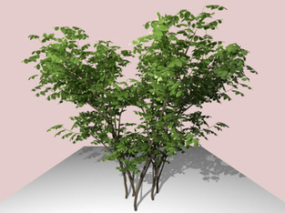 |
| Figure 25.2
Synthetic plant (dogrose) with Lattice Boltzmann lighting.
|
A visualization of the Lattice Boltzmann lighting alone is shown in
Figure 25.3
. Here each fragment is colored with the three-component photon density from the nearest grid node. The virtual sun is located on the left. This produces significant mid-band illumination that causes the right side to appear darker than the left. Thus, we are capturing both transmission and ambient occlusion.
 |
| Figure 25.3
Visualization of Lattice Boltzmann lighting for the dogrose plant.
|
The key parameter values here were derived from the values reported in the remarkable study by Knapp and Carter
[19]
that showed that the reflective and transmissive properties of plants are essentially constant across species. The wavelength-dependent values used are shown in
Table 25.1
. Visible energy loss due to absorption was modeled by zeroing out the
f
0
component at each site on each iteration.
The reflective and transmissive properties of polymethyl methacrylate (PMMA) are well known. It is a lightweight, shatter-resistant alternative to glass that is often used in automobile taillights. To push the limits of our lighting technique, we fashioned a (hypothetical) PMMA teapot and applied LB lighting. The results are shown in
Figure 25.4
. The key model parameter values are shown in
Table 25.2
.
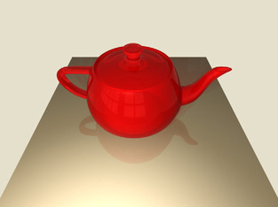 |
| Figure 25.4
Lattice Boltzmann lighting for the PMMA teapot.
|
| Red | Green | Blue | |
|---|---|---|---|
| Henyey – Greenstein g | 0.80 | −0.88 | −0.88 |
| σ a | 0.01 | 0.01 | 0.01 |
| σ s | 0.99 | 0.99 | 0.99 |
Although the effects of LB lighting here are admittedly minimal, we find that it offers a small, but believable “glow” that is not available with conventional lighting. In
Figure 25.5
we show the same teapot, rendered with conventional lighting, where the ambient surface color is set equal to the diffuse surface color.
 |
| Figure 25.5
The PMMA teapot with conventional lighting.
|
25.4. Final Evaluation
In
Table 25.3
we compare timings for solutions of our LB lighting model as applied to the 256 × 128
2
grid used in the cloud lighting example of
Section 25.3.2
. Because each line includes a 1-second CPU overhead for loading, the available speedup (without resorting to SSE instructions or multithreading) is from 1169 s to 5 s, or 234x.
It is interesting to note that by resorting to SSE instructions and multithreading on the i7 X980, we can achieve an execution time that is better than that of the naive kernel running on the GTX 480.
Results scale linearly with available resources. It should be expected that doubling the longest edge dimension would increase execution time by a factor of four. There are twice as many nodes, but achieving steady-state requires twice as many iterations. In
Table 25.4
we show execution times for a cloud model of size 128
3
. Results are as expected. Of the 2 seconds required for the final kernel on the 128
3
problem, approximately 0.7 seconds may be attributed to CPU loading, and thus the expected factor of ×4 holds for all entries.
Although the computational structure of our method is similar to that which would be used in a parallel implementation of the discrete ordinates method, it is important to remember that our simulation-like structure is actually a numerical solution of an approximating diffusion equation. Thus, like Stam's approach
[27]
, its value is probably restricted to highly scattering geometry. Nevertheless, on the other side of this same coin, one should not expect any ray effects, as seen in the discrete ordinates derivatives.
We believe that our LB lighting model is effective in quickly lighting scenes with highly scattering geometry, such as clouds or forests. It is best used to capture diffuse transmission, interobject scattering, and ambient occlusion, all of which are important to photo-realism.
There are limitations. Because the technique models photon transport as a diffusion process, it is inappropriate for most direct illumination effects. Thus, it must be augmented with other techniques to capture such effects. Another limitation is the memory requirement. Because the grid state is maintained as floats:
cl_mem focl[2][WIDTH*HEIGHT*DEPTH*DIRECTIONS];
a grid of size 256
3
would require 2.5 GB, and larger grids would exceed available GPU memory. To light a scene with more than a single cloud or a single tree and yet capture interobject, indirect illumination requires a grid hierarchy, such as the one suggested in
[28]
.
25.5. Future Directions
More effective use of grids of limited size is under investigation. The impressive real-time performance achieved by Kaplanyan and Dachsbacher
[17]
can be attributed to their use of nested grids of varying resolution positioned in camera space. Their grid hierarchy is more sophisticated than our own
[28]
and could offer significant performance benefits. Another approach is the use of dynamic grids. In
[5]
we proposed a spring-loaded vertex model for 2-D radiosity computations. The grids were represented as point masses interconnected by zero-rest-length springs. Spring forces were dynamically determined by the current best lighting solution until equilibrium, with an attendant deformed grid, was achieved. This approach allowed high-quality lighting solutions with relative small grid sizes. Application of this approach to 3-D lighting appears most promising.
25.6. Derivation of the Diffusion Equation
The purpose of this section is to show that, as the lattice spacing,
λ
, and the time step,
τ
, both approach 0, the limiting behavior of the fundamental update in
Eq. 25.2
is the diffusion
Eq. 25.3
. A sketch of the derivation originally appeared in
[11]
. The present treatment includes significantly more detail. As noted earlier, the principal value of this derivation is as a prototype for related derivations.
We begin by expanding the left side of
Eq. 25.2
in a Taylor series with respect to the differential operator
 which handles three spatial dimensions and one temporal. This gives us

(25.10)
(25.11)
For the diffusion behavior we seek, it will be important for the time step to approach 0 faster than the lattice spacing. Specifically, we write
 that is,
t
0
is a term that approaches 0 faster than
ϵ
2
, and
that is,
t
0
is a term that approaches 0 faster than
ϵ
2
, and
 It follows from the chain rule for differentiation that
 and
and
 As is standard practice in Lattice Boltzmann modeling, we also assume that we can write
 as a small perturbation on this same scale about some local equilibrium,
f
(0)
, i.e.,
as a small perturbation on this same scale about some local equilibrium,
f
(0)
, i.e.,
 where the local equilibrium carries the total density, i.e.,
 .
Equation 25.12
is the Chapman-Enskog expansion from statistical mechanics
[4]
, wherein it is assumed that any flow that is near equilibrium can be expressed as a perturbation in the so-called Knudsen number,
ϵ
, which represents the mean free path (expected distance between successive density collisions) in lattice spacing units.
.
Equation 25.12
is the Chapman-Enskog expansion from statistical mechanics
[4]
, wherein it is assumed that any flow that is near equilibrium can be expressed as a perturbation in the so-called Knudsen number,
ϵ
, which represents the mean free path (expected distance between successive density collisions) in lattice spacing units.
(25.12)
Equation 25.11
now becomes:
(25.13)
Equating coefficients of
ϵ
0
in
(25.13)
, we obtain:
 i.e.,
f
(0)
is indeed a local equilibrium. In general, a local equilibrium need not be unique, and the choice can affect the speed of convergence
[18]
. Nevertheless, in this case it turns out that Ω has a one-dimensional null space. We observe that
i.e.,
f
(0)
is indeed a local equilibrium. In general, a local equilibrium need not be unique, and the choice can affect the speed of convergence
[18]
. Nevertheless, in this case it turns out that Ω has a one-dimensional null space. We observe that
 (where entries 1–6 are 1/12) satisfies
 , all
m
, and so we must have
, all
m
, and so we must have
 where the scaling coefficient,
K
, is determined by the requirement that
where the scaling coefficient,
K
, is determined by the requirement that
 . Thus, we have:
(25.14)
(25.15)
Similarly, equating coefficients of
ϵ
1
in (25.13
), we obtain:
 that is, after substituting
Eq. 25.15
,
that is, after substituting
Eq. 25.15
,
 We would like to solve
Eq. 25.17
for
f
(1)
, but we cannot simply invert Ω, since it is singular. Nevertheless, we can observe that any vector comprising lattice direction components,
We would like to solve
Eq. 25.17
for
f
(1)
, but we cannot simply invert Ω, since it is singular. Nevertheless, we can observe that any vector comprising lattice direction components,
 as well as any of
 is an eigenvector of Ω with eigenvalue −
σ
t
. Thus, if we write
is an eigenvector of Ω with eigenvalue −
σ
t
. Thus, if we write
 and substitute into (25.17
), we can determine that
K
= −
λ
/((1 +
σ
a
)
σ
t
) and so
and substitute into (25.17
), we can determine that
K
= −
λ
/((1 +
σ
a
)
σ
t
) and so
(25.16)
(25.17)
(25.18)
Finally, we need to equate
ϵ
2
terms in
Eq. 25.13
, but here it will suffice to sum over all directions. We obtain:
 Substituting
(25.15)
and
(25.18)
into
Eq. 25.19
and observing that
Substituting
(25.15)
and
(25.18)
into
Eq. 25.19
and observing that
 we obtain
 which, if we multiply through by
ϵ
2
, yields the standard diffusion equation,
which, if we multiply through by
ϵ
2
, yields the standard diffusion equation,
 with diffusion coefficient
 The critical step is clearly a choice of Ω that both represents plausible collision events and has readily determined eigenvectors that can be used to solve for the first few components in the Chapmann-Enskog expansion.
(25.19)
(25.20)
(25.21)
Acknowledgments
This work was supported in part by the National Science Foundation under Award 0722313 and by an equipment donation from NVIDIA Corporation.
References
[1]
J. Arvo,
Transfer equations in global illumination
,
In:
Global Illumination, SIGGRAPH ’93 Course Notes
,
vol. 42
(1993
)
.
[2]
N. Bhate, A. Tokuta,
Photorealistic volume rendering of media with directional scattering
,
In:
Third Eurographics Workshop on Rendering
(1992
)
Bristol
, pp.
227
–
245
.
[3]
S. Chandrasekhar,
Radiative Transfer
. (1950
)
Clarendon Press
,
Oxford
.
[4]
B. Chopard, M. Droz,
Cellular automata modeling of physical systems
. (1998
)
Cambridge University Press
,
Cambridge
.
[5]
R. Danforth, R. Geist,
Automatic mesh refinement and its application to radiosity computations
,
Int. J. Robot. Autom.
15
(1
) (2000
)
1
–
8
.
[6]
D. d’Humières, P. Lallemand, U. Frisch,
Lattice gas models for 3d hydrodynamics
,
Europhys. Lett.
2
(1986
)
291
–
297
.
[7]
C. Donner, H. Jensen,
Light diffusion in multi-layered translucent materials
,
ACM Trans. Graph.
24
(3
) (2005
)
1032
–
1039
.
[8]
R. Fattal,
Participating media illumination using light propagation maps
,
ACM Trans. Graph.
28
(1
) (2009
)
1
–
11
.
[9]
J.R. Frisvad, N.J. Christensen, H.W. Jensen,
Computing the scattering properties of participating media using Lorenz-Mie theory
,
In:
SIGGRAPH ’07: ACM SIGGRAPH 2007
(2007
)
ACM
,
New York
, pp.
60-1
–
60-10
.
[10]
M. Gardner,
Mathematical games: John Conway's game of life
,
Sci. Am.
223
(1970
)
120
–
123
.
[11]
R. Geist, K. Rasche, J. Westall, R. Schalkoff,
Lattice-Boltzmann lighting
,
In:
Rendering Techniques 2004 (Proc. Eurographics Symposium on Rendering)
Norrkőping, Sweden
. (2004
), pp.
355
–
362
;
423
.
[12]
R. Geist, J. Steele,
A lighting model for fast rendering of forest ecosystems
,
In:
Proceeding of the IEEE Symposium on Interactive Ray Tracing (RT08), Los Angeles, CA
(2008
), pp.
99
–
106
;
(also back cover)
.
[13]
R. Geist, J. Steele, J. Westall,
Convective clouds
,
In:
Natural Phenomena 2007 (Proceeding of the Eurographics Workshop on Natural Phenomena), Prague, Czech Republic
(2007
), pp.
23
–
30
;
83 (and back cover)
.
[14]
G. Henyey, J. Greenstein,
Diffuse radiation in the galaxy
,
Astrophys. J.
88
(1940
)
70
–
73
.
[15]
H. Jensen, S. Marschner, M. Levoy, P. Hanrahan,
A practical model for subsurface light transport
,
In:
Proceedings of SIGGRAPH 2001
(2001
)
ACM
,
New York
, pp.
511
–
518
.
[16]
J. Kajiya, B. von Herzen,
Ray tracing volume densities
,
ACM Comput. Graph. (SIGGRAPH ’84)
18
(3
) (1984
)
165
–
174
.
[17]
A. Kaplanyan, C. Dachsbacher,
Cascaded light propagation volumes for real-time indirect illumination
,
In:
I3D ’10: Proceedings of the 2010 ACM SIGGRAPH Symposium on Interactive 3D Graphics and Games
(2010
)
ACM
,
New York
, pp.
99
–
107
.
[18]
I. Karlin, A. Ferrante, C. Ottinger,
Perfect entropy functions of the lattice boltzmann method
,
Europhys. Lett.
47
(1999
)
182
–
188
.
[19]
A. Knapp, G. Carter,
Variability in leaf optical properties among 26 species from a broad range of habitats
,
Am. J. Bot.
85
(7
) (1998
)
940
–
946
.
[20]
E. Languénou, K. Bouatouch, M. Chelle,
Global illumination in presence of participating media with general properties
,
In:
Fifth Eurographics Workshop on Rendering
Darmstadt, Germany
. (1994
), pp.
69
–
85
.
[21]
N.L. Max,
Efficient light propagation for multiple anisotropic volume scattering
,
In:
Fifth Eurographics Workshop on Rendering
Darmstadt, Germany
. (1994
), pp.
87
–
104
.
[22]
P.M. Binvox,
http://www.cs.princeton.edu/~min/binvox/binvox.html
(2003
)
.
[23]
F. Nooruddin, G. Turk,
Simplification and repair of polygonal models using volumetric techniques
,
IEEE Trans. Visual. Comput.
9
(2
) (2003
)
.
[24]
Greenworks Organic-Software, Xfrogplants v 2.0
http://www.xfrogdownloads.com/greenwebNew/products/productStart.htm
(2008
)
.
[25]
H. Rushmeier, K. Torrance,
The zonal method for calculating light intensities in the presence of a participating medium
,
In:
Proceeding SIGGRAPH ’87
(1987
)
ACM
,
New York
, pp.
293
–
302
.
[26]
X. Shan, G. Doolen,
Multicomponent lattice-boltzmann model with interparticle interaction
,
J. Stat. Phys.
81
(1/2
) (1995
)
379
–
393
.
[27]
J. Stam,
Multiple scattering as a diffusion process
,
In:
Proceeding of the 6th Eurographics Workshop on Rendering, Dublin, Ireland, Eurographics Association
Aire-la-Ville, Switzerland
. (1995
), pp.
51
–
58
.
[28]
J. Steele, R. Geist,
Relighting forest ecosystems
,
In: (Editor: G. Bebis,
et al.
)
ISVC 2009 Part I, LNCS 5875 (Proceedings of the 5th International Symposium on Visual Computing), Las Vegas, NV
(2009
)
Springer
,
Heidelberg
, pp.
55
–
66
.
[29]
N. Thürey, U. Rüde, M. Stamminger,
Animation of open water phenomena with coupled shallow water and free surface simulations
,
In:
SCA ’06: Proceedings of the 2006 ACM SIGGRAPH/Eurographics Symposium on Computer animation, Vienna, Austria, Eurographics Association
Aire-la-Ville, Switzerland
. (2006
), pp.
157
–
164
.
[30]
A. Watt, M. Watt,
Advanced animation and rendering techniques: Theory and practice
. (1992
)
Addison-Wesley
,
Wokingham, England
.
[31]
X. Wei, W. Li, K. Mueller, A. Kaufman,
The Lattice-Boltzmann method for gaseous phenomena
,
IEEE Trans. Visual. Comput.
10
(2
) (2004
)
.
..................Content has been hidden....................
You can't read the all page of ebook, please click here login for view all page.