
Chapter 45. ℓ1 Minimization in ℓ1-SPIRiT Compressed Sensing MRI Reconstruction
Mark Murphy and Miki Lustig
Magnetic resonance imaging (MRI) is a rich, multidisciplinary topic whose modern success is due to a synthesis of knowledge from many fields: medicine, physics, chemistry, engineering, and computer science. This chapter discusses the successful Cuda parallelization of an algorithm (ℓ 1-SPIRiT
[5]
: ℓ 1-regularized
iT
erative
S
elf-consistent
P
arallel
I
maging
R
econstruction) for reconstructing MR images acquired using two advanced methods: compressed sensing and parallel imaging (CS+PI).
The issues discussed in this chapter are simlilar to those faced by many MRI and statistical signal processing applications. Computationally, ℓ 1-SPIRiT requires solving many independent convex optimization problems, each of which is a substantial computational burden on its own. All algorithms for solving the optimization problems are iterative, requiring repeated application of several linear operators that implement interpolations and orthonormal transformations.
45.1. Introduction, Problem Statement, and Context
The acquisition of MR images in clinical contexts is inherently slow. MRI examinations are long and uncomfortable for patients; they also are expensive for hospitals to provide. MRI is an incredibly flexible imaging modality with many medical applications. The lengthiness and expense of MRI exams limits MRI's applicability in many contexts, however. MRI scans are inherently slow for two reasons. First, MRI data must be sampled sequentially, and each sample is expensive. An MRI scanner produces discrete samples of k-space
1
one at a time by applying a series of time-varying magnetic fields in the presence of a very strong constant magnetic field. There are unavoidable physical limits on the rate of change of these magnetic fields, as well as the rate at which the molecules in the patient's body can respond to the fields. Second, MRI is plagued by an inherently low signal-to-noise ratio (SNR). If too little time is spent acquiring the MRI data, then the image will be dominated by the unavoidable noise generated by the MR system and the patient's body.
1
In MRI and related fields, the Fourier-domain representation of an image is usually called “k-space.”
Compressed sensing (CS) is an approach to ameliorating the first cause: A CS MRI scan simply acquires fewer data points. However, as we will discuss briefly, one must be careful to acquire the
right
data points. Parallel imaging (PI) ameliorates the second cause: redundantly acquiring the MR data from multiple receive channels improves the signal-to-noise ratio. With PI, one can effectively trade SNR for scan time. In either case, ℓ 1-SPIRiT's approach to combining these two techniques can substantially increase the quality and speed of MR imaging. Although combining CS+PI results in less MRI data being collected, we still desire high-resolution images. Thus, ℓ 1-SPIRiT must estimate the values of the data that weren't collected.
Typically, SPIRiT is applied to 3-D volumetric scans acquired redundantly from 8–32 receive channels. In resolution, each of the dimensions varies between 128 and 512, and we undersample by approximately 4×. Each voxel is a single-precision complex number, and these datasets range in size from hundreds of MB to several GB. The iterative algorithms for performing SPIRiT reconstruction, combined with the massive datasets, produce long runtimes that threaten SPIRiT's clinical usability. The original research prototype of ℓ 1-SPIRiT requires over an hour to reconstruct these images. However, a radiologist directing an MRI examination must have the images from each scan before prescribing the next: the reconstruction must execute “instantaneously.” As we will discuss in later sections, our implementation of ℓ 1-SPIRiT reconstructs these MRI scans in fewer than 30 seconds on a multi-GPU system, running faster even than serial implementations of competing, simpler techniques. The code described in this chapter has been deployed at Lucile Packard Children's Hospital, and is used to reconstruct dozens of scans per week. C++ source code is available on-line from the author's Web site:
http://www.eecs.berkeley.edu/~mjmurphy/llspirit/html
.
45.1.1. Compressed Sensing
Compressed sensing
[4]
is a general approach for reconstructing a signal when it has been sampled significantly below the Nyquist rate. To develop intuition of the usefulness and mechanics of compressed sensing,
Figure 45.1
provides a detailed example of its application to a toy signal. In this section, we provide a brief treatment of the mathematical formalism.
 |
| Figure 45.1
A simple example of a compressed sensing recontsruction. Panel A shows a length-128 signal
y
, which we wish to sample below the Nyquist rate. Panel B shows ŷ, a random subsampling of
y
at
|
First, we must discuss
sparsity
. A vector
x
is considered
sparse
if it has very few nonzero elements. A vector itself that is not sparse may be sparse when represented via some other basis. This will occur, for example, when the vector is simply a linear combination of a few of the vectors in the basis. For example a sine wave is not sparse, but has a very compact representation in the Fourier domain. Some vectors may not be sparse, but may be
compressible
— the magnitudes of their coefficients in some basis decay rapidly. Such a vector is nearly sparse, except for a large number of small coefficients.
In MRI, we wish to produce an image of the density of tissues on a patient's body. We can denote an image as
 : an
n
-dimensional complex-valued vector.
n
is the number of voxels in our 3-D images — typically 100 million or more. Using the MRI scanner we want to take
m
samples of the k-space (i.e., Fourier domain) representation of our image, with
m
≪
n
to accelerate the scan. We can represent the process of taking these measurements as multiplication of
x
with a matrix Φ, constructed by selecting some subset of the rows of a discrete Fourier transform (DFT) matrix. We'll denote the undersampled k-space data
y
= Φ
x
. Because
m
≪
n
, the problem of inverting the equation
y
= Φ
x
is highly underdetermined: a solution can be drawn from an entire (m
−
n
)-dimensional subspace of ℂ
n
.
: an
n
-dimensional complex-valued vector.
n
is the number of voxels in our 3-D images — typically 100 million or more. Using the MRI scanner we want to take
m
samples of the k-space (i.e., Fourier domain) representation of our image, with
m
≪
n
to accelerate the scan. We can represent the process of taking these measurements as multiplication of
x
with a matrix Φ, constructed by selecting some subset of the rows of a discrete Fourier transform (DFT) matrix. We'll denote the undersampled k-space data
y
= Φ
x
. Because
m
≪
n
, the problem of inverting the equation
y
= Φ
x
is highly underdetermined: a solution can be drawn from an entire (m
−
n
)-dimensional subspace of ℂ
n
.
Real-world images such as the ones produced by MRI tend to be compressible: image compression algorithms such as JPEG
[6]
leverage this fact. In particular JPEG uses a wavelet transform to expose compressibility, as real-world images tend to be nearly sparse in the wavelet domain. Compressed sensing provides a means of selecting a particular solution
 (of the many which satisfy Φ
x
=
y
): the image which is maximally sparse. Formally, our desired image can be found by solving the following optimization problem:
(of the many which satisfy Φ
x
=
y
): the image which is maximally sparse. Formally, our desired image can be found by solving the following optimization problem:
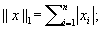
 Where the ℓ 1 norm is defined as the sum of the absolute value of a vector's components:
 and
Wx
is the representation of
x
in a wavelet basis. The compressed sensing reconstruction problem is convex, and thus, it is possible to design tractable algorithms for its solution
[3]
. However, these algorithms will necessarily be iterative and, given the large size of our datasets, very computationally expensive.
and
Wx
is the representation of
x
in a wavelet basis. The compressed sensing reconstruction problem is convex, and thus, it is possible to design tractable algorithms for its solution
[3]
. However, these algorithms will necessarily be iterative and, given the large size of our datasets, very computationally expensive.
45.1.2. Parallel Imaging
Parallel Imaging (PI) refers to the redundant acquisition of an MR image from multiple receive coils. Parts of the patient's body closer to a given coil will produce a stronger signal in that coil, so the 8–32 receive coils in a PI acquisition are arranged to provide good coverage of an entire region of the body. Because each coil receives a high signal-to-noise ratio (SNR), the scan can be performed substantially faster — frequently in 2 – 4× less time. Each channel produces only a partial image, but much of the volume is imaged redundantly from the many coils. The SPIRiT reconstruction leverages this redundancy as an additional constraint in the ℓ 1 minimization required by compressed sensing.
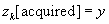
In particular, given a nonacquired k-space location
x
(i
,
j
,
k
), SPIRiT computes a set of weights to be applied to all k-space voxels within some radius (typically 2–3 voxels) surrounding
x
(i
,
j
,
k
). The value of the nonacquired k-space location is estimated as the sum of the weights times the neighboring voxels from all coils’ images — i.e., missing k-space data are estimated by convolving the known data with a shift-invariant filter. However, the undersampling pattems used by SPIRiT produce adjacent missing k-space data. Thus, SPIRiT seeks a fixed point of this convolution operation: i.e., a set of estimates for the missing k-space data that is self-consistent with respect to these interpolation kernels.
More formally, because convolution is a linear operation we can represent the application of interpolation kernels to an image
x
as a linear transformation
Gx
. We'll refer to
G
as the “Calibration Operator” because it encodes all information about our multicoil calibration. The self-consistency formulation is equivalent to requiring that
x
be a fixed point of
G
:
Gx
=
x
. We can further constrain the compressed sensing problem with this additional linear equality, producing the final specification of the ℓ 1-SPIRiT reconstruction:
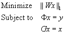
(45.1)
45.2. Core Methods (High Level Description)
In this section, we discuss the algorithm we currently use to solve the ℓ 1-SPIRiT reconstruction in
Equation 45.1
. Our algorithm is a “Projections-Over-Convex-Sets” (POCS) method. That is, we iteratively apply projections onto three convex sets corresponding to the three terms in
Equation 45.1
: images which are “wavelet sparse” (i.e., ||
Wx
||
1
is small); images which are “Measurement Consistent” (i.e., Φ
x
=
y
); and images which are “calibration consistent” (i.e.,
Gx
−
x
). The POCS algorithm is most succinctly described in pseudocode:
do {
k
= k + 1
(1)
 % Enforce calibration consistency
(2)
 % Enforce Data consistency
(3)
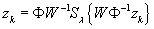 % Wavelet soft-threshold
} until convergence
The three lines marked (1
), (2
), and (3
) are the sources of computational intensity in the algorithm. Here we have used
z
k
to denote the k-space representation of the image,
G
and Φ as the Calibration and Fourier operators, and
W
as the wavelet transform operator, thus the effect of lines (1
) and (2
) should be clear. We have used
S
λ
to denote a
soft-thresholding
operation.
S
λ
is defined elementwise on a vector as
 That is,
S
λ
(x
i
has the same phase as
x
i
, but a slightly smaller magnitude. The effect of soft thresholding is to remove wavelet coefficients owing to aliasing resulting from the k-space undersampling: thus, the soft-thresholding removes aliasing noise and prevents image artifacts from appearing.
That is,
S
λ
(x
i
has the same phase as
x
i
, but a slightly smaller magnitude. The effect of soft thresholding is to remove wavelet coefficients owing to aliasing resulting from the k-space undersampling: thus, the soft-thresholding removes aliasing noise and prevents image artifacts from appearing.
45.3. Algorithms, Implementations, and Evaluations (Detailed Description)
Most of the computation involved in the algorithm described in the previous section manifests itself as simple elementwise operations on the image data. Given the availability of the highly optimized CUFFT library, the parallelization and optimization of our code is fairly straightforward. The exception is the wavelet transform, which required substantially more optimization than the other operations.
Our MRI pulse sequence only undersamples the data in two of the three dimensions. Undersampling in the first dimension, the
readout direction
, is not sensible. This is a consequence of the use of gradient fields by MRI scanners to manipulate k-space: acquiring an entire readout line is no more expensive than acquiring a single point along that line. Consequently, we can decouple the 3-D problem into many independent 2-D problems by performing an inverse Fourier transform along the readout direction. Each independent 2-D problem can be solved in parallel. Each 2-D problem itself is a substantial computation, and our implementation parallelizes the 2-D solver across a single GPU. In systems with multiple GPUs, we distribute 2-D problems round-robin to ensure load balance.
45.3.1. Calibration Consistency Operator
As described in
Section 45.2
, the application of the Calibration Consistency operator
G
is a convolution in the Fourier domain. It is well known that convolutions in the Fourier domain are equivalent to elementwise multipication in the image domain. If the convolution kernel has
m
coefficients, and the image has
n
voxels, then the the implementation of
G
in the Fourier domain is
O
(mn
), while the implementation in the Image domain is only
O
(n
) after incurring an
O
(n
log
n
) cost of performing Fourier transforms. Note that we must perform the Fourier transforms anyway — otherwise, we could not compute the wavelet transform and perform the soft-thresholding operation. Thus, the Fourier transforms effectively cost nothing, and an image domain implementation is clearly more efficient. Furthermore, convolutions are more difficult to optimize than elementwise operations, and we can more easily produce a near-peak-performance image-domain implementation.
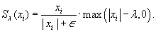
Figure 45.2
shows an example of the image-domain elementwise masks that are used to compute the Fourier-domain convolutions.
 |
| Figure 45.2
An example 2-D slice of four channels of a brain MRI, and the image-domain masks used to implement the k-space calibration-consistency convolution efficiently. To estimate the nonacquired k-space samples for a given channel, each pixel in the images on the left would be multiplied by the four weights from the desired row of mask images.
|
However, the image-domain implementation requires a substantially higher memory footprint than does the Fourier-domain implementation. In the Fourier domain, the convolution kernels are very small. Each kernel is typically 7
3
, and we have typically 8 × 8 of them. However, to represent these kernels in the image domain, we must zero-pad them to the size of the image (at least 128
3
) and perform an inverse Fourier transform. This increasess memory usage by approximately three orders of magnitude: we must carefully manage this data, or we will overrun the memory capacity of the GPUs.
If there are eight channels in the MRI acquisition (typically there are eight, but there can be as many as 32), then we have 64 convolution kernels. For a typical volume size of 384 × 256 × 100 with eight channels, precomputing and all of the image-domain masks would require 384 × 256 × 100 × 8 × 8 complex-valued, single-precision: 4.6 GB of data. For a 32-channel acquisition, this would balloon to 75 GB. However, because the 3-D problem decouples into independent 2-D problems, we need to store the image-domain covolution masks only for as many 2-D problems as we have in flight simultaneously. Currently, we have one 2-D problem in flight per GPU in the system. This may change in future versions of the code, however, as we will discuss in
Section 45.5
. For each 256 × 100 2-D problem of a 32-channel acquisition, the 2-D convolution masks require 200 MB of memory and fit in the DRAM of any reasonably sized CUDA-capable GPU.
Our implementation of the calibration consistency operator uses neither the texture cache, nor the shared memory because there is little data reuse that can be exploited. All data (the convolution masks and the image data itself) are stored in the GPU's DRAM and streamed through using standard coalesced memory operations. Because the code performs just under 1 complex floating-point operation per complex float loaded from DRAM, the computation rapidly becomes DRAM bandwidth bound and no further optimization is necessary.
45.3.2. Data Consistency Projection
The data consistency projection serves the purpose of ensuring that our estimate of the image does not diverge from the data produced during the MRI scan. Our implementation of this projection is simple. First we transform our current estimate
x
k
into the Fourier domain, for which we use the highly optimized CUFFT libary. The Fourier transform of our estimate will include “estimated” values for the k-space voxels acquired from the MRI scan. However, we know that these estimates are wrong: these k-space voxels should have the values produced by the MRI scan. Thus, the second step of the data-consistency projection is simply to overwrite these voxels with the known values.
Much as in the case of the Calibration Consistency projection, this step is trivially parallel and rapidly becomes bandwidth bound. Furthermore, the bulk of the work is in computing the Fourier transforms. As discussed in
Section 45.5
, reliance on CUFFT in this step has overly constrained our current parallelization of the SPIRiT algorithm possibly leading to substantial inefficiency.
45.3.3. Soft Thresholding
As discussed in
Section 45.2
, the soft-thresholding step can be intuitively understood as a denoising operation that decreases the ℓ 1 norm of the wavelet representation of the image. This step has the effect of pushing to zero wavelet coefficients that are very small and consolidating the energy of the signal about a sparse set of coefficients. In our context, we consider the magnitude of a wavelet coefficient to be the sum across all 8–32 channels of the magnitude of the channels’ individual wavelet coefficients. Our implementation serializes the sum for each voxel, instead exploiting the more abundant voxel-wise parallelism. After computing the sum, we can compute what the new magnitude should be for each wavelet coefficient and update in place the data.
Much as in the implementation of the data-consistency and calibration-interpolation operations, little optimization is needed in order to achieve efficient execution. Soft thresholding is very easily written via standard CUDA programming practice to achieve near-peak memory bandwidth utilization. Because the runtime of this step is dominated by memory access, and no reuse can be exploited, we need not optimize the code any further.
45.3.4. Wavelet Transform
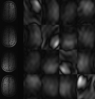
Figure 45.3
shows an example of the application of a wavelet transform to an MR image. The forward and inverse wavelet transforms are the most intricately optimized steps of our implementation. The algorithm we are using to compute the wavelet transforms in ℓ 1-SPIRiT is
O
(n
lg
n
) (n
is the number of pixels in the image) and repeatedly convolves the image with high- and low-pass filters, downsampling at every step. The result is a spatial separation of the image content corresponding to high- and low-frequency Fourier coefficients. The algorithm performs
O
(lg
n
) steps, during which the image undergoes several
O
(n
) convolutions.
 |
| Figure 45.3
On the left is a typical MRI image. The center is the image after one step of a wavelet transform. Note that the image has been spatially high-pass filtered in both X and Y and downsampled to produce the bottom-right quarter; low-pass filtered in both X and Y for the top-left quarter; and a combination of high- and low-pass filtering was used to produce the other two quarters. On the right is the image after four steps of the wavelet transform.
|
If during one step of a wavelet transform, the image is
H
pixels tall and
W
pixels wide
2
, our goal is to produce four
H
/2 by
W
/2 pixel images, one of which is high-pass filtered in both the X and Y dimensions, one of which is low-pass filtered in both dimensions, and two which are a combination of low- and high-pass filtered in the two dimensions. This could be achieved by performing four 2-D convolutions, and downsampling by a factor of two. However, a more efficient implementation leverages the separability of the wavelet filters. In particular, the 2-D convolutions are performed as pairs of 1-D convolutions: first convolving each length
W
row with high- and low-pass filters, then convolving each length
H
column. The downsampling operation can be combined with the convolution to reduce computation by a factor of 2×.
2
Our implementation is of a
dyadic
wavelet, requiring that both the width and height be zero-padded to powers of two so that downsampling by a factor of two is always legal.
While we are performing a convolution on a row (or column) of the image, it is crucial to cache the input data to leverage the data reuse inherent in convolution. We are using length-
P
(usually four) filters and performing two down-sampling convolutions, so effective caching will reduce memory bandwidth requirements by a factor of
P
×. Again, we expect that an efficient implementation of the wavelet transform should be memory bound owing to the extremely high floating-point throughput of the GPU. Note that when we are convolving in the nonunit stride dimension (in our case, convolving the rows of the image), it is also necessary to block in the unit-stride dimension. In order for memory accesses to be coalesced, we must load up to 16 rows at a time into the GPU's shared memory. In fact, we found that blocking increased the performance of both our row and column convolutions, likely because of the increased thread block size the blocking transformation enabled. Once the blocked data is in shared memory, we can then perform our convolutions rapidly on the cached data.
The implementations of the row- and column-convolutions for both the forward and inverse transforms are similar. Here, we provide a partial listing of the source for the forward transform's row convolution, with some details omitted for clarity. Note that the
shared_rows
variable represents the data we are caching in the GPU's shared memory, and the constant
K
determines how many rows we load into a single thread block's memory. Because the data is column major,
K
must be large enough to ensure that global memory accesses are coalesced. The high- and low-pass filters are stored in the GPU's constant memory in arrays named
hpf
and
lpf
, respectively. Also, note that while the MRI data is complex valued, our wavelet filters are real valued. Thus, we perform the transform independently on the real and imaginary components of the data.
 |
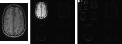
| Figure 45.4. |
| Illustration of the convolutions performed during the wavelet transform. The horizontal and vertical lines on the left are convolved with a quadrature-pair of high- and low-pass filters and downsampled to produce the corresponding portions of the images on the right. In order for the GPU hardware to coalesce the memory accesses for the row-convolutions, we must combine the convolutions for at least eight rows into a single thread block and load the resulting image strip into shared memory. The same blocking transformation also improves the columnwise convolutions (which are unit stride, and would coalesce anyway) by increasing thread-block size.
|
_ _global_ _ void forward_wavelet_rows ()
{
// some initializaion omitted for bevity
extern _ _shared_ _ float shared_rows[];
for (int j = threadIdx.y; j < n; j += blockDim.y)
shared_rows[threadIdx.x + j*blockDim.x] = X[i + M*j];
__syncthreads();
// Low-pass Downsample
for (int j = threadIdx.y; j < n/2; j += blockDim.y){
float y = 0;
for (int k = 0; k < P; k++)
y += shared_rows[threadIdx.x + K*(2*j+k)&(n-1)]*lpf[k];
X[i + j*M] = y;
}
// High-pass Downasmple
for (int j = threadIdx.y; j < n/2; j += blockDim.y){
float y = 0;
for (int k = 0; k < P; k++)
y += shared_rows[threadIdx.x + K*mod(2*j+1-k,n)]*hpf[k];
X[i + (n/2)*M + j*M] = y;
}
This code parallelizes the computation of each row's convolution among
 of the threads in a thread block. Since
K
rows are loaded, the entire thread block computes
K
convolutions in parallel. However, a wavelet transform of a single image is insufficient to saturate the GPU for any appreciable amount of time. Additional parallelism is found in performing the transforms for all 8–32 channels simultaneously. Additionally, our wavelet filters are real valued and transforms of the complex-valued MRI images further decompose into real and imaginary transforms which can be performed in parallel.
of the threads in a thread block. Since
K
rows are loaded, the entire thread block computes
K
convolutions in parallel. However, a wavelet transform of a single image is insufficient to saturate the GPU for any appreciable amount of time. Additional parallelism is found in performing the transforms for all 8–32 channels simultaneously. Additionally, our wavelet filters are real valued and transforms of the complex-valued MRI images further decompose into real and imaginary transforms which can be performed in parallel.
void forward_wavelet (float *X_real, float *X_imag, int M, int N, C, int L)
{
T = 256; // threads per Thread Block
int min_size = (1 ≪ L);
// other variable initializaion omitted for clarity
for (int m = M, n = N, j = J, j > L; j−−)
{
if (m > min_size)
{
for (K = MAX_K
; K*m*sizeof(float) > SHARED_MEM_SIZE
; K ≫= 1);
forward_wavelet_cols ⋘ dim3(2, C*(n/K)), dim3(T/K, K) K*m*sizeof(float) ⋙ (X_real, X_imag, M, m, N, n, C);
}
if (n > min_size)
{
for (K = MAX_K
; K*n*sizeof(float) > SHARED_MEM_SIZE
; K ≫= 1);
forward_wavelet_rows ⋘ dim3(2*(m/K), C), dim3(K, T/K), K*n*sizeof(float) ⋙ (X_real, X_imag, M, m, N, n, C);
}
if (m > min_size) m = m/2;
if (n > min_size) n = n/2;
}
In the preceding code, we have called the column and row convolutions as separate kernels: all convolutions are performed in place in global DRAM, and the output of the column convolutions is the input to the row convolutions. The grid dimensions of
dim3(2,C*(n/K))
and
dim3(2*(m/k),C)
specify that we want to perform convolutions for all
C
image channels in parallel, that we are grouping the
n
column convolutions (or
m
row convolutions) into groups of
K
, and we multiply by two in order to process the real and imaginary components separately.
45.4. Final Evaluation and Validation of Results, Total Benefits, and Limitations
The original research prototype implementation of ℓ 1-SPIRiT was a Matlab script, relying on Matlab's efficient implementations of Fourier transforms and matrix/vector operations, as well as an external C implementation of wavelet transforms. Our CUDA implementation is 100 to 200 times faster than this code, although the comparison is hardly fair. Instead, we shall use an optimized C++ implementation as a performance baseline, running on the CPU cores of our reconstruction machine. Our reconstruction machine is a dual-socket Intel Xeon X5650 Westmere system, with six dual-threaded cores per socket running at 2.67 GHz. The six cores in each socket share a 12 MB L3 cache, and have private 256kB L2 caches and 64kB Ll caches. The machine also has four Tesla C1060 GPGPUs in PCI Express x16 slots. Each Tesla C1060 has 240 single-precision execution pipelines running at 1.3 GHz, organized into 30 streaming multiprocessors (SMs), with 4 GB of dedicated graphics DRAM capable of approximately 100 GB/s bandwidth. Each of the 30 SMs has a 16kB shared scratchpad memory accessible by all threads in the SM, and a 64kB register file partitioned among threads. All CUDA tools used were version 2.3. All non-CUDA C++ code was compiled with GNU G++ 4.3.3.
We'll discuss the runtime of ℓ 1-SPIRiT for three different high-resolution eight-channel 3-D acquisitions.
Table 45.1
summarizes several important characteristics of these datasets. The “Seq. ℓ 1-Min Time” column reports the runtime of our optimized C++ code running on a single core of the recon machine. The “#2-D Problems” column is the readout dimension, which determines the number of independent 2-D reconstructions that must be performed. Dataset A is typical of a very high-resolution scan, typically performed of a pediatric patient's abdomen under general anesthesia. Scans B and C are typical resolutions for other applications, for example in 4-D Flow
[2]
, where the scan resolution is lower but a large number (approximately 100) of individual 3-D volumes are acquired over a period of time. 4-D Flow reconstructions require each individual 3-D volume to be reconstructed, and total reconstruction time can be many hours.
The end-to-end MRI reconstruction requires some computations not discussed in the previous sections. For all datasets, there are approximately 11 seconds of runtime not spent
int
the POCS iterations: 7 seconds solving linear systems of equations to produce the calibration operator
G
, 3 seconds performing Fourier transforms of the readout direction, and the remaider in miscellaneous minor computations. Because of space limitations, we shall not discuss these computations further.
Table 45.2
compares the runtimes of our various parallel implementations of the ℓ 1 minimization code. It is worth noting that our one-CPU implementation is fairly well optimized: this code itself is approximately 4× faster than the original Matlab implementation. The “12CPUs” column is the same source code as the one-CPU implementation, but parallelized using OpenMP
[1]
. In all cases, the CPU parallelization is fairly efficient. The smaller two datasets, B and C, achieve 10× speedup using 12 CPU cores.
Interestingly, although the hyperthreading on the Intel Nehalem architecture can provide approximately a 30% performance boost for some codes, in this case, using more than 12 CPU threads substantially hurts performance — increasing runtime by approximately 50% for problem A. This effect is due to contention for cache and memory bandwidth. The large caches on the CPU platform are in large part responsible for the good scaling of the CPU code: note that the smaller problems (B and C) scale more efficiently on the CPU than does the larger problem (A). The size of the 2-D datasets for B and C are 1.1 and 0.95 MB, respectively. Most operations in the algorithm are out of place, so two copies of the data must be allocated. With 12 2-D problems in flight simultaneously, and a working set size of about 2 MB per problem, the algorithm will run almost entirely in the 24 MB of CPU cache in the system.
However, the GPU implementation scales better for the large dataset (A). Our GPU implementation is 50% more efficient for dataset (A) than for dataset (B). This effect is due to synchronization overhead and GPU utilization. The larger problem is simply more work, with longer average runtimes for all kernels and less frequent pipeline flushes owing to global synchronizations. Given that the small shared memories are not sufficient to cache the large 2 MB working set, almost all computations must stream their inputs and outputs to/from the GPU's DRAM. As discussed in the previous section, memory bandwidth is the most important microarchitectural resource for all of this algorithm's operations. If there is not enough concurrency to adequately compensate for the large DRAM access latency, performance will suffer. This is precisely the reason for the relative inefficiency of the GPU parallelization.
45.5. Discussion and Conclusion
In the previous section, we discussed how our GPU implementation is more efficient with larger problem sizes, as smaller problems are less capable of saturating the GPU's execution and memory access pipelines. This leads one to wonder why we did not implement the reconstruction so that multiple 2-D problems could be in flight simultaneously on each GPU. The “one problem per GPU” decision is due to the relative inflexibility of the CUFFT 2.3 API. In particular, in CUFFT 2.3 2-D transforms cannot be batched, and they cannot be non-unit stride. Additionally, the CUFFT optimized routines can be called only from the CPU host, rather than from inside device code. As a result of these restrictions, the only practical way to perform Fourier transforms in our context is to “serialize” our many 2-D transforms, and allow CUFFT to leverage the moderate parallelism within each transform. FFTs require substantial synchronization, and our 2-D FFTs are not very large — in particular, the size of the 2-D problems listed in
Table 45.1
. Thus, the FFTs are relatively inefficient.
One particularly interesting alternate parallelization strategy is to execute each 2-D problem in a single thread block. Each 2-D problem typically requires less than 100 MB of DRAM, and the GPU's global memory capacity can easily support hundreds of 2-D problems in flight simultaneously. A 32-channel problem requires substantially more memory, but would still allow for nearly full occupancy, especially if the memory footprint is reduced by implementing the calibration interpolation in the Fourier-domain, as discussed in
Section 45.3.1
.
The recently released CUFFT 3.0 allows batched FFTs of any dimensionality, via the
cufftPlanMany
API. Thus, we could have many 2-D Fourier transforms in flight simultaneously; however, the 2-D problems must synchronize at least twice per iteration: the CUFFT routines can be called only from the CPU host, and two transforms (forward and inverse) are preformed per iteration. Thus, CUFFT presents a middle-ground solution that could provide higher FFT performance, but still require frequent global syncrhonizations.
Despite the inefficiency of the current parallelization strategy, the 40 × speedup for the largest (and most important) datasets has proven sufficient for clinical applicability of the ℓ 1-SPIRiT technique. Our software has been deployed in a clinical setting for six months at the time of this writing and has reconstructed thousands of MRI scans. The largest of datasets, e.g., dataset A in
Table 45.1
, reconstruct in under a minute, and most datasets reconstruct in 20–30 seconds. Such runtimes are short enough that the radiologist prescribing scans will scarcely notice them.
References
[1]
OpenMP: an API for shared-memory parallel programming in C/C++ and FORTRAN,
http://www.openmp.org
.
[2]
M.T. Alley, P.J. Beatty, A. Hsiao, S.S. Vasanawala,
Reducing the scan time of time-resolved, 3d phase contrast imaging with 2d autocalibrated parallel imaging
,
In:
ISMRM
(2010
)
.
[3]
S. Boyd, L. Vandenberghe,
Convex Optimization
. (2004
)
Cambridge University Press
.
[4]
E. Candes, J. Romberg, T. Tao,
Robust uncertainty principles: exact signal reconstruction from highly incomplete frequency information
(2004
)
.
[5]
M. Lustig, J.M. Pauly,
SPIRiT: iterative self-consistent parallel imaging reconstruction from arbitrary k-space
,
Magn. Reson. Med.
(2010
)
.
[6]
M.W. Marcellin, M.J. Gormish, A. Bilgin, M.B. Boliek,
An overview of JPEG-2000
(2000
)
.
..................Content has been hidden....................
You can't read the all page of ebook, please click here login for view all page.