
Chapter 46. Medical Image Processing Using GPU-Accelerated ITK Image Filters
Won-Ki Jeong, Hanspeter Pfister and Massimiliano Fatica
46.1. Introduction
In this chapter we introduce GPU acceleration techniques for medical image processing using the insight segmentation and registration toolkit (ITK)
[1]
. ITK is one of the most widely used open-source software toolkits for segmentation and registration of medical images from CT and MRI scanners. It consists of a collection of state-of-the-art image processing and analysis algorithms that often require a lot of computational resources. Although many image processing algorithms are data-parallel problems that can benefit from GPU computing, the current ITK image filters provide only limited parallel processing for certain types of image filters. The coarse-grain parallel multithreading model employed by the current ITK implementation splits the input image into multiple chunks and assigns a thread for each piece, taking advantage of the capabilities of multiprocessor shared-memory systems (Figure 46.1
). However, the performance increase as the number of cores grows is sublinear owing to memory bottlenecks.
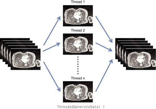 |
| Figure 46.1
Coarse-grain parallelism implemented in current ITK image filters.
|
Because many ITK image filters are embarrassingly parallel and do not require interthread communication, we can exploit the fine-grain data parallelism of the GPU
[4]
. To validate these ideas we implemented several low-level ITK image processing algorithms, such as convolution, statistical, and PDE-based de-noising filters, using NVIDIA's CUDA. We have two main goals in this work:
• Outlining a simple and easy approach to integrate CUDA code into ITK with only minimal modification of existing ITK code
• Demonstrating efficient GPU implementations of spatial-domain image processing algorithms.
We believe that our approach gives developers a practical guide to easily integrate their GPU code into ITK, allowing researchers to use GPU-accelerated ITK filters to accelerate their research and scientific discovery.
46.2. Core Methods
We implemented three widely used spatial-domain image processing algorithms
[2]
: linear convolution, median filter, and anisotropic diffusion (Figure 46.2
).
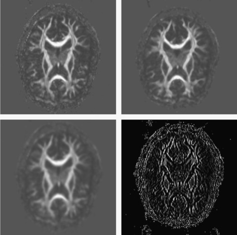 |
| Figure 46.2
ITK image filtering results. Top left: Input image. Top right: Median filter. Bottom left: Gaussian filter. Bottom right: Magnitude of gradient filter.
|
Linear convolution
Linear convolution is the process of computing a linear combination of neighboring pixels using a predefined set of weights, that is, a weight
mask
, that is common for all pixels in the image (Figure 46.3
). The Gaussian, mean, derivative, and Hessian of Gaussian ITK filters belong to this category. Linear convolution for a pixel at location (x
,
y
) in the image
I
using a mask
K
of size
M
×
N
is computed as:
 where
I
new
is the new image after filtering. Assuming without loss of generality that the domain is a two-dimensional image, the mask
K
is symmetric along the
x
and
y
axis, and
M
and
N
are odd numbers, then
a
= (M
− 1)/2, and
b
= (N
− 1)/2.
Figure 46.3
shows the linear convolution process in the image domain using a 3 × 3 mean filter mask as an example.
where
I
new
is the new image after filtering. Assuming without loss of generality that the domain is a two-dimensional image, the mask
K
is symmetric along the
x
and
y
axis, and
M
and
N
are odd numbers, then
a
= (M
− 1)/2, and
b
= (N
− 1)/2.
Figure 46.3
shows the linear convolution process in the image domain using a 3 × 3 mean filter mask as an example.
(46.1)
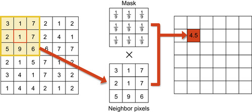 |
| Figure 46.3
Linear convolution with a mean filter mask.
|
This type of filter maps very effectively to the GPU for several reasons. First, convolution is an embarrassingly data-parallel task because each pixel value can be independently computed. We can assign one GPU thread per pixel, and there is no interthread communication during the computation. Second, the same convolution mask
K
is applied to every pixel, leading to SIMD (single instruction multiple data)-friendly computation. Last, only adjacent neighbor pixels are used for the computation, leading to highly spatial coherent memory access. See
Section 46.3.2
for implementation details.
Median filter
The ITK median filter belongs to the category of statistical filters where the new pixel value is determined based on the local nonlinear statistics; that is, the median of neighboring pixels. The filter is mainly used to remove salt-and-pepper noise while preserving or enhancing edges (Figure 46.2
). Although each pixel value can be computed independently, computing nonlinear statistics is not a GPU-friendly task. We overcome this problem by employing a bisection search technique that can be implemented more efficiently on the GPU than naive per-pixel histogram computation (see
Section 46.3.3
).
Anisotropic diffusion
The anisotropic diffusion filter we implemented solves a gradient-based nonlinear partial differential equation (PDE) first introduced by Perona and Malik
[5]
. The filter mimics the process of heat dispersion in inhomogeneous materials to remove image noise while preserving important features. The PDE is defined as follows:
 The amount of diffusion per pixel is anisotropically defined by the diffusivity term
c
(x
). This is a fall-off function; for example,
The amount of diffusion per pixel is anisotropically defined by the diffusivity term
c
(x
). This is a fall-off function; for example,
 applied to the gradient magnitude ||∇
I
|| at each pixel. There are several different implementation variants of Perona and Malik's diffusion PDE, but we follow the approach proposed in the original paper. In order to solve the PDE we discretize the equation using a finite difference method and employ an iterative Euler integration method to calculate the solution. Our GPU numerical solver can be applied to a wide range of partial differential equations (see
Section 46.3.4
).
applied to the gradient magnitude ||∇
I
|| at each pixel. There are several different implementation variants of Perona and Malik's diffusion PDE, but we follow the approach proposed in the original paper. In order to solve the PDE we discretize the equation using a finite difference method and employ an iterative Euler integration method to calculate the solution. Our GPU numerical solver can be applied to a wide range of partial differential equations (see
Section 46.3.4
).
(46.2)
46.3. Implementation
In this section, first we will describe how to integrate GPU code written in NVIDIA CUDA into existing ITK code. Then, we will discuss the GPU implementation details of each ITK image filter.
46.3.1. Integration of NVIDIA CUDA Code into ITK
To integrate GPU code into ITK we needed to modify some common ITK files and add new files into the ITK code base. We have edited or added source code into the
Code/BasicFilters
and
Code/Common
directories and added a new directory
Code/CUDA
where all CUDA source code (.cu) as well as related headers are located. Two new functions,
checkCUDA()
and
initCUDA()
, are introduced to check the availability of a GPU and to initialize it, respectively.
Our approach to integrate CUDA code into ITK is to make it transparent to the users so that any application program written using the previous ITK library does not need to be modified. To use GPU functionality the application code needs only to be re-compiled and linked against our new ITK library. To selectively execute either CPU or GPU versions of the ITK filters, the user sets the operating system environment variable
ITK_CUDA
accordingly. The entry points for each ITK image filter are the new member functions
ThreadedGenerateData()
(for multithreaded filters) or
GenerateData()
(for single-threaded filters) that implement the actual filter operations. Inside these functions we check the
ITK_CUDA
flag using the
checkCUDA()
function to branch the execution path to either the CPU or GPU at runtime.
Figure 46.4
shows a code snippet of
ThreadedGenerateData()
in
itkMean-ImageFilter.txx
that shows how existing ITK filters can be modified to selectively execute GPU or CPU code.
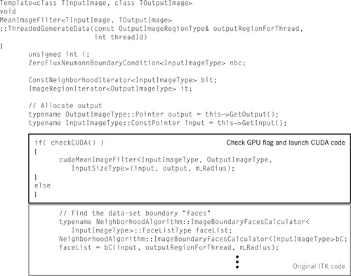 |
| Figure 46.4
Code snippet of the modified
itkMeanImage Filter.txx
that incorporates CUDA code.
|
Each GPU filter consists of host code written in C++ that runs on the CPU with calls to the CUDA runtime and GPU kernel code written in CUDA that is called by the host code. When a GPU ITK filter is launched, the host code dynamically allocates GPU memory, copies the input ITK image and filter parameters to GPU memory (e.g.,
input
,
output
, and
m_Radius
in
Figure 46.4
), and launches the GPU kernel to perform the actual computation. Once kernel execution has finished, the host code copies the results from GPU memory to the output ITK image.
In the GPU kernel code we have to pay special attention to dealing with different pixel formats and input image dimensions. The current CUDA ITK implementation can handle two- and three-dimensional images and 8-bit unsigned char or 32-bit float pixel types. In older versions of CUDA, each type of conversion has to be explicitly done by implementing a separate GPU kernel for each possible input and output pixel type. However, this limitation no longer exists in the newer CUDA compilers (version 3.0 and beyond) that support C++ templates.
We now describe the details of the GPU data structures and parallel algorithms for the different image filters discussed in
Section 46.2
.
46.3.2. Linear Convolution Filters
The linear convolution filters we implemented — mean, Gaussian, derivative, and Hessian of Gaussian — are separable. Therefore, an
n
-dimensional convolution can be implemented as a product of one-dimensional convolutions along each axis, which reduce the per-pixel computational complexity from
O
(m
n
) to
O
(nm
), where
m
is the kernel size along one axis and
n
is the dimension of the input image. We implemented a general one-dimensional CUDA convolution filter and applied it along each axis successively using the corresponding filter mask weights.
For a filter mask of size
n
, there are 2
n
memory reads (n
mask reads,
n
neighbor pixel value reads), and 2
n
− 1 floating-point operations (n
multiplications and
n
− 1 addition). Because a global memory fetch instruction is more expensive compared with a single floating-point instruction and there are roughly the same number of memory and floating-point instructions, our problem is memory bound. Therefore, we mainly focus on optimizing memory access in our GPU filter implementation.
Data layout
The convolution filters use local neighbors to compute the weighted average, and each pixel is used multiple times by its neighbors. Therefore, bringing spatially close pixel values into the fast GPU shared memory or texture cache and sharing them between threads in the same thread block reduces global memory bandwidth. In our filter implementations we use shared memory. In addition, the filter mask is identical for every pixel. We precompute the filter mask weights in the host code and copy them to the GPU's constant memory so that all GPU threads can share it via a cache.
To further minimize the data transfer time between global and shared memory, we configure the dimension of the CUDA thread block such that adjacent kernels do not overlap.
Figure 46.5
(upper row) shows an example of splitting the domain into regular-shaped blocks, which results in additional global memory access in the region where kernels overlap (between the dotted lines). Instead, we can split the domain into elongated blocks (bottom left) to eliminate kernel overlap (bottom right).
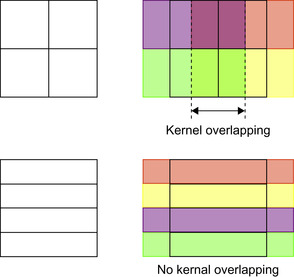 |
| Figure 46.5
Kernels overlap on regular shaped blocks (top). No kernel overlapping on elongated blocks (bottom). Rectangles on the left column are CUDA blocks. Shaded rectangles on the right column are memory regions to be copied to shared memory for each block.
|
Filter weight computation
The weights for a mean filter mask are 1/(kernel size) and the one-dimensional Gaussian weights are normalized (e.g., (0.006, 0.061, 0.242, 0.383, 0.242, 0.061, 0.006) for unit standard deviation). We use central-difference weights (0.5, 0, −0.5) and (0.25, −0.5, 0.25) for the first and second derivative filters, respectively. The Hessian of Gaussian filter computes the second derivatives of the Gaussian. For example, a 3-D Hessian of Gaussian matrix is defined as follows:
 Each tensor component is the second derivative of the image convolved with a Gaussian filter mask. This can be naively implemented by successively applying Gaussian and derivative filters. However, it is better to combine two convolutions into a single convolution filter because the combination of two separable filters is also separable. Therefore, each tensor component can be computed by applying the corresponding 1-D convolution filter along each axis. For example,
 can be computed by applying a 1-D second-order derivative of Gaussian filter along the
x
-axis followed by applying a 1-D Gaussian filter along the
y
and
z
axes. The weights for the 1-D derivative Gaussian filter can be calculated algebraically, as shown in
Figure 46.6
.
can be computed by applying a 1-D second-order derivative of Gaussian filter along the
x
-axis followed by applying a 1-D Gaussian filter along the
y
and
z
axes. The weights for the 1-D derivative Gaussian filter can be calculated algebraically, as shown in
Figure 46.6
.
 |
| Figure 46.6
Computing weights for the zero-, first-, and second-order derivatives of a Gaussian filter.
|
46.3.3. Median Filter
The median filter is a nonlinear statistical filter that replaces the current pixel value with the median value of pixels in the neighboring region. A naive implementation first creates a cumulative histogram for the neighbor region and then finds the first index beyond half the number of pixels in the histogram. The major problem of this approach on the GPU is that each thread needs to compute a complete histogram, and therefore 256 histogram bins have to be allocated per pixel for an 8-bit image. This is inefficient on current GPUs because there are not enough hardware registers available for each thread, and using global memory for histogram computation is simply too slow.
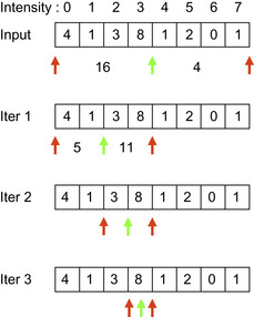
To avoid this problem, our implementation is based on a bisection search on histogram ranges proposed in
[6]
. This method does not compute the actual histogram but iteratively refines the histogram range that includes the median value. During each iteration, the current valid range is divided into two halves, and the half that has the larger number of pixels is chosen for the next round. This process is repeated until the range converges to a single bin. This approach requires log
2
(number of bins) iterations to converge. For example, an image with an 8-bit pixel depth (256 bins) requires only eight iterations to compute the median.
Figure 46.7
shows an example of this histogram bisection scheme for eight histogram bins.
 |
| Figure 46.7
A pictorial example (left) and pseudocode (right) of the histogram bisection scheme. This example is based on eight histogram bins (i.e., 3 bits per pixels). Left: Dark grey arrows indicate the current valid range, and the light grey arrow (described as
pivot
in the pseudocode on the right) indicates the location of the median bin.
|
Because we do not want to store the entire histogram but want to keep track of only a valid range for each thread, we have to scan all the neighbor pixels in each iteration to refine the range. This leads to a computational complexity of
O
(m
log
2
n
), where
n
is the number of histogram bins (a constant for a given pixel format) and
m
is the number of neighboring pixels to compute the median (a variable depending on the filter size). To minimize the
O
(m
) factor, we store neighboring pixels in shared memory and reuse them multiple times. Similar performance can be achieved using texture memory instead of shared memory.
46.3.4. Anisotropic Diffusion Filter
A numerical solution of
Equation 46.2
can be calculated using a standard finite difference method
[3]
, where time discretization is approximated by a forward explicit Euler method as follows:
 We approximate the right side of
Equation 46.3
using one-sided gradients and conductance values defined at the center of adjacent pixels (light grey crosses in
Figure 46.8
). The solution can be computed by iteratively updating the image using the following formula (for the 2-D case):
We approximate the right side of
Equation 46.3
using one-sided gradients and conductance values defined at the center of adjacent pixels (light grey crosses in
Figure 46.8
). The solution can be computed by iteratively updating the image using the following formula (for the 2-D case):
 where
I
±
are one-sided gradients computed using forward/backward differences along an axis. For example, the one-sided gradients at the pixel location (i
,
j
) along the
x
-axis can be computed as follows:
where
I
±
are one-sided gradients computed using forward/backward differences along an axis. For example, the one-sided gradients at the pixel location (i
,
j
) along the
x
-axis can be computed as follows:
 where
h
x
is the grid spacing along the
x
-axis (Figure 46.8
).
where
h
x
is the grid spacing along the
x
-axis (Figure 46.8
).
(46.3)
(46.4)
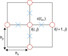 |
| Figure 46.8
The grid setup for the derivative approximation and conductance computation in the 2-D case. The circles are pixel values, and crosses are conductance values defined in the middle between adjacent pixels.
|
Each pixel value is used multiple times — for example, four times for 2-D and six times for 3-D — to compute the one-sided gradients and conductance values. We precompute the one-sided gradients and conductance values per pixel and store them in shared memory to eliminate redundant computation and to reduce global memory access. The preprocessing step is done per block right before the actual Euler integration in the same CUDA kernel. Note that
I
x
+
(i
,
j
) =
I
x
−
(i
+ 1,
j
). Therefore, we need to precompute only one one-sided gradient image per axis instead of computing all forward and backward gradients. For example, for an
n
×
n
2-D block, we first copy (n
+ 2) × (n
+ 2) pixels (current block and its adjacent neighbor pixels) from global to shared memory and then compute four (n
+ 1) × (n
+ 1) lookup tables for forward gradients and conductance values for the
x
and
y
directions, respectively. We thereby reduce not only the shared memory footprint but also the computation time by half. Backward gradients and their conductance values can be accessed by simply shifting the index by −1.
We use the Jacobi method to iteratively update the solution. In the Jacobi method, each pixel can be independently processed without communicating with others, mapping naturally to the GPU's massively parallel computing model. For each update iteration we use a source and a target buffer. The GPU kernel is allowed to read only from the source buffer and to write only to the target buffer to ensure data consistency. Because a single iteration is running a GPU kernel, the new result must be written back to global memory at the end of each GPU kernel call. The time step
dt
needs to be set properly so that the iterative process does not diverge. In our experience
dt
= 0.25 for 2-D and
dt
= 0.16 for 3-D work well.
46.4. Results
We tested our GPU ITK filters on a Windows PC equipped with an NVIDIA Quadro FX 5800 GPU, two Intel Xeon Quad-core (total eight cores) CPUs running at 3.0 GHz, and 16 gigabytes of main memory. We used NVIDIA CUDA 2.3 and ITK 3.12 to build the GPU ITK filters. Although this is a first attempt to assess the usability of current GPUs to accelerate existing ITK code, the results look very promising. We measure wall clock time for each filter execution, including CPU-to-GPU data transfer times, to compare the actual application-level performance. Timings are measured in seconds for a 256 × 256 × 256 3-D volume dataset. Our GPU ITK filters on a single GPU are up to 45 times faster than the multithreaded ITK filters on
eight
CPU cores.
We observed the biggest speedup for the anisotropic diffusion filter. As clearly visible in
Figure 46.9
, the iterative Jacobi update on a regular grid is an embarrassingly parallel task, resulting in a huge speedup on the GPU. In addition, we have observed that the current ITK anisotropic diffusion filter does not scale well to many CPU cores (only up to 4× speedup on eight CPU cores).
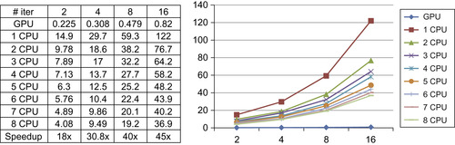 |
| Figure 46.9
Running time comparison of the anisotropic diffusion filter.
|
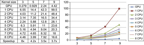
Convolution filters also map well on the GPU.
Figure 46.10
shows the running times of the ITK discrete Gaussian filter and our GPU implementation. The GPU version runs up to 19 times faster than the CPU version on eight CPU cores. In addition, the GPU version runs much faster for large kernel sizes because more processor time is spent on computation rather than I/O. Similar to the anisotropic filter, the current ITK Gaussian filter does not scale well to multiple CPU cores.
 |
| Figure 46.10
Running time comparison of the Gaussian filter.
|
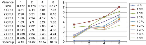
Finally, our GPU median filter runs up to eight times faster than the current ITK median filter (Figure 46.11
). Because statistical filters cannot be easily parallelized on SIMD architectures, the performance of our GPU median filter is acceptable. In addition, the GPU version is still roughly 20× faster if it is compared with the result on a single CPU core.
 |
| Figure 46.11
Running time comparison of the median diffusion filter.
|
In summary, we demonstrated that GPU computing can greatly boost the performance of existing ITK image filters. In addition, we introduced a simple approach to integrate CUDA code into the existing ITK code by modifying the entry point of each filter. Using only a single GPU easily beats eight CPU cores for all tests we performed, thus confirming the great potential of GPUs for highly parallel computing tasks. The current implementation is open source and can be downloaded at
http://sourceforge.net/projects/cudaitk/
and used freely without any restriction for non-commercial use.
46.5. Future Directions
Although our prototype GPU ITK filters have shown promising results, we have found several fundamental problems in the current implementation that may degrade their efficiency in a more complicated setup. First, our GPU implementation does not provide a native ITK GPU image class or data structure that supports the pipelining of ITK filters — a common strategy in ITK workflows. Therefore, in the current implementation, the entire image data must be copied between CPU and GPU memory at the end of each filter execution. This may become a significant bottleneck for pipelining multiple filters for large images because the data must travel through the PCI-e bus repeatedly. Developing a new ITK native GPU image class that supports pipelining on GPU memory would solve this issue. Another problem is that the current ITK image filters had to be rewritten from scratch to run on the GPU because easy-to-use GPU template code is not readily available. Another target for future work will be GPU image filter templates or operators that provide basic functions to access and manipulate image data and that may help developers to easily implement additional GPU filters.
46.6. Acknowledgments
This work was supported in part by the National Science Foundation under Grant No. PHY-0835713 and through generous support from NVIDIA. Won-Ki Jeong accomplished this work during his summer internship at NVIDIA in 2007.
[1]
The Insight Segmentation and Registration Toolkit
http://www.itk.org
(2010
)
.
[2]
R.C. Gonzalez, R.E. Woods,
Digital image processing
.
second ed.
(2006
)
Prentice-Hall
,
Saddle River, NJ
.
[3]
K.W. Morton, D.F. Mayers,
Numerical solution of partial differential equations: an introduction
. (2005
)
Cambridge University Press
,
New York
.
[4]
J.D. Owens, D. Luebke, N. Govindaraju, M. Harris, J. Krger, A.E. Lefohn,
et al.
,
A survey of general-purpose computation on graphics hardware
,
Comput. Graph. Forum
26
(1
) (2007
)
80
–
113
.
[5]
P. Perona, J. Malik,
Scale-space and edge detection using anisotropic diffusion
,
IEEE Trans. PAMI
12
(7
) (1990
)
629
–
639
.
[6]
I. Viola, A. Kanitsar, M.E. Groller,
Hardware-based nonlinear filtering and segmentation using high-level shading languages
,
In: (Editors: G. Turk, J.J. van Wijk, R.J. Moorhead)
Proceedings of the 14th IEEE Visualization 2003 (VIS'03), 19–24 October 2003
Seattle, WA, IEEE Computer Society, Washington, DC
. (2003
), p.
41
.
..................Content has been hidden....................
You can't read the all page of ebook, please click here login for view all page.