
Chapter 48. Multiscale Unbiased Diffeomorphic Atlas Construction on Multi-GPUs
Linh Ha, Jens Krüger, Sarang Joshi and Cláudio T. Silva
In this chapter, we present a high-performance multiscale 3-D image-processing framework to exploit the parallel processing power of multiple graphic processing units (multi-GPUs) for medical image analysis. We developed GPUs algorithms and data structures that can be applied to a wide range of 3-D image-processing applications and efficiently exploit the computational power and massive bandwidth offered by modern GPUs. Our framework helps scientists solve computationally intensive problems that previously required supercomputing power. To demonstrate the effectiveness of our framework and to compare it with existing techniques, we focus our discussions on atlas construction –the application of understanding the development of the brain and the progression of brain diseases.
48.1. Introduction, Problem Statement, and Context
48.1.1. Atlas Construction Problem
The construction of population atlases plays a central role in medical image analysis, particularly in understanding the variability of brain anatomy. The method projects a large set of images to a common coordinate system, creating a statistical average model of the population, and doing regression analysis of anatomical structures. This average serves as a deformable template that maps detailed atlas data, such as structural, developmental, genetic, pathological, and functional information, on to the individual or entire population of the brain. This transformation encodes the variability of the population understudy. Likewise, the statistical analysis of the transformation between populations reflects the interpopulation differences. Apart from providing a common coordinate system, the atlas can be partitioned and labeled, thus providing effective segmentation via registration of anatomical labels.
The brain atlas construction is a powerful technique to study the physiology, evolution, and development of the brain, as well as disease progression. Two desired properties of the atlas construction are that it should be diffeomorphic and nonbiased.
In nonrigid registration problems, the desired transformations are often constrained to be diffeomorphic, that is, continuous, one to one (invertible), and smooth with a smooth inverse so that the topology is maintained. Connected sets remain connected; disjoint sets remain disjoint; neighbor relationships between structures, as well as smoothness of features, such as curves, are preserved; and coordinates are transformed consistently.
Preserving topology is important for synthesizing the atlas because the knowledge base of the atlas is transferred to the target anatomy through topology preserving transformation providing automatic labeling and segmentation. Moreover, important statistics such as the total volume of a nucleus, the ventricles, or the cortical subregion can be generated automatically. The diffeomorphic mapping from the atlas to the target can be used to study the physical properties of the target anatomy, such as mean shape and variation. Also, the registration of multiple individuals to a standard atlas coordinate space removes the individual anatomical variation and allows information to be combined with a single conical anatomy.
Figure 48.1
shows that the diffeomorphic setting results in a high-quality deformation field that is infinitely smooth on a non-self-crossing grid.
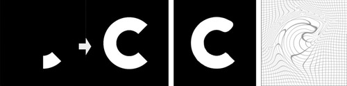 |
| Figure 48.1
A small part of the letter “C” deforming into a full “C” using 2-D greedy iterative diffeomorphism. From left to right: (1) Input and target image. (2) Deformed template. (3) Grid showing the deformation applied to the template.
|
The nonbias property guarantees that the atlas construction is consistent. Our atlas construction framework, first proposed by Joshi
et al.
[9]
, is based on the notion of Frechet mean to define a geometrical average. On a metric space
 , with a distance
 the intrinsic average
 of a collection of data
 is defined as a minimizer of the sum-of-square distances to each individual, that is
As the computation of the Frechet mean is independent from the order of the inputs, the atlas is inherently nonbiased. The Frechet mean is also rational in terms of minimizing the total energy to deform an average to all images in a population.
The combination of both diffeomorphic and nonbias property results in a minimization energy template problem which is formulated as
 subject to
 (*)
(*)
(48.1)
1:
Input
:
 volume inputs
2:
Output
: Template atlas volume
3:
for
 to
to
 do
do
4:
Fix images
 , compute the optimal template

5:
for
 to
to
 do
{loop over the images}
do
{loop over the images}
6:
Fix the template
 , solve pairwise-matching problem between
 and
and

7:
Update the image with optimal velocity field
8:
end for
9:
end for
This is a dual-optimization problem on the image matching (the first term) and deformation energy (the second term). The
 -operator is a partial differential operator that controls the smoothness of the deformation field. The constraint (*) comes from the theory of large deformation diffeomorphism that the transformations
 are generated by integrating velocity field
 forward in time. The method is the extension of elastic registration to handle large deformations.
Although the optimization seems intractable, by noting that for fixed transformation
 the best estimation of the average
 is given by
 , we come up with a simple solution based on an alternating optimization, as shown on
Algorithm 1
. In each step, we estimate the atlas by averaging the deformed images, then compute the optimal velocity fields by solving optimization problems on deformation energy, and finally update the deformed images. This process is repeated until convergence. Note that, with the assumption of a fixed template on the second step, the optimal velocity of an image can be computed independently from the others. This velocity is determined by solving the pairwise matching problem. By tightly coupling the atlas construction problem with basic registration problems — the pairwise matching algorithms — our framework allows us to implement different techniques and even to combine multiple techniques into a hybrid approach.
, we come up with a simple solution based on an alternating optimization, as shown on
Algorithm 1
. In each step, we estimate the atlas by averaging the deformed images, then compute the optimal velocity fields by solving optimization problems on deformation energy, and finally update the deformed images. This process is repeated until convergence. Note that, with the assumption of a fixed template on the second step, the optimal velocity of an image can be computed independently from the others. This velocity is determined by solving the pairwise matching problem. By tightly coupling the atlas construction problem with basic registration problems — the pairwise matching algorithms — our framework allows us to implement different techniques and even to combine multiple techniques into a hybrid approach.
48.1.2. Challenges
As shown in the preceding section, unbiased diffeomorphic atlas construction is a powerful method in computational anatomy. However, the impact of the method was limited because of two main challenges: the extensive memory requirement and the intensive computation.
The extensive memory requirement is one of the major obstacles of 3-D volume processing in general because the size of a single volume often exceeds the available memory on a processing node. This becomes more challenging on GPUs because they have less memory available. In addition, the atlas construction process requires not just a single volume, but a population of hundreds of volumes, thus easily exceeding the available memory of pratically any computational system.
The massive size of the problem is compounded with the complexity of the computation per element. These computations are often not just simple local kernels, but global operations, for example, an ODE integration using a backward mapping technique.
Generating a brain atlas at an acceptable resolution for a reasonably sized population took an impractically long time even with a fully optimized implementation on high-end CPU workstations
or small CPU clusters
[6]
. Acceptable run times could only be obtained by utilizing supercomputer resources
[3]
and
[4]
. Hence, the technique was restricted to the baseline research community. Fortunately, the development of GPUs in recent years, especially the introduction of a general processing model and a unified architecture, brings a more accessible solution. Our results show that an implementation on the GPU can handle practical problems on a single desktop with a substantial performance gain, on the order of 20 to 60 times faster than a single CPU.
Our multi-GPU implementation on a 32-node GPU cluster is roughly 1000 times faster than a 32-core CPU workstation. We are able to handle a large dataset of 315 T1 brain images at size
 using only eight cluster nodes. The ability to solve the problem on small-scale computing systems opens opportunities for researchers to fully understand practical impacts of the method and to enhance their knowledge of anatomical structures.
In addition to providing a practical solution to a specific problem, we also present a general image processing framework and optimization techniques to exploit the massive bandwidth and computational power of multi-GPU systems and to handle compute-expensive problems previously available only on a supercomputer.
Although we have integrated a number of different techniques into our system, such as the greedy iterative diffeomorphism, large deformation diffeomorphic metric mapping (LDDMM), and metamorphoses, in this chapter we focus on the implementation of the greedy method on GPUs.
48.2. Core Methods
The greedy iterative diffeomorphism was proposed by Christensen
[5]
. The method separated the time dimension from the space dimension of the problem. At each iteration, a new optimal velocity field is computed, given that the current deformation is fixed (i.e., the past velocity fields are fixed). The solution is computed by integrating the optimal solution at each step forward in time in a gradient descent approach. The method is locally in-time optimal; thus, in general, it will not produce the shortest path connecting images through the space of diffeomorphism. However, it is generally preferred in practice because it can produce good results with less computational expense than the other approaches. The greedy iterative diffeomorphism is built on the general framework with the greedy pairwise matching algorithm at its core (Algorithm 2
).
There are several performance keys of a GPU implementation: high-throughput data structures and basic functions; high-performance advance functions, such as optimal ODE integration and PDE solvers; and multiresolution and multi-GPU strategies. We will discuss in detail how to achieve the peak performance in the following section.
48.3.1. Data Structures
Although it is typically recommended to have volume data padding so that the volume dimensions are multipliers of the GPU warp size, our experiment showed that it has a negligible effect on improving the performance. The reason is that as GPU data-parallel fetching strategies become more sophisticated and efficient, the coalesced condition is greatly relieved from CUDA 1.0 to CUDA 2.0 hardware, so it is easy to achieve with regular image functions. Moreover, data padding significantly increases the storage requirement, especially in 3-D, and requires extra processing steps. For these reasons, we chose a tight 3-D volume representation that can represent a 3-D volume as a 1-D vector; thus, most of the basic operations on 1-D can be directly applied to 3-D. Additionally, we often save two integer shared-memory locations and operations per kernel by passing a single-volume value instead of three-dimensional numbers.
We also define a special structure for 3-D vector fields based on a structure of array representation. Instead of allocating three separated GPU pointers, we allocate a single memory block and use an offset to address the three components. This presentation allows us to optimize basic operations on the vector field, most of the time as a single-image operation. Moreover, it helps us save one shared-memory pointer per kernel.
48.3.2. Basic Image Operators
The goal of our system design is to be able to run the entire processing pipeline on GPUs. This allows one to maximize the computational benefit from GPUs and minimizes idle time. We keep data flow running on the GPUs and use only CPUs for cross-GPU and cross-CPU operations. With the design goal in mind to be optimal, even on a per-function level, we provide n-ary basic-3-D functions.
The performance of the basic function is constrained by the global memory bandwidth. To improve the performance we need to minimize the bandwidth usage. Most of the functions provided by regular processing libraries such as Thrust
[8]
or NPP (http://developer.nvidia.com/object/npp_home.html
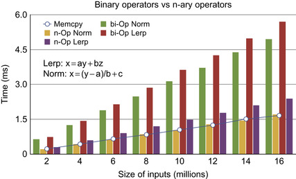
) are unary or binary functions that involve one or two arguments as the inputs. Although any n-argument function can always be decomposed into a set of unary and binary functions, this decomposition requires extra memory to store intermediate results, and increases bandwidth utilization by saving and/or reloading the data. Our n-ary operators, on the other hand, load all the components of an n-argument function to the register files at the same time; hence, no extra saving/loading is required. This process allows for optimal memory bandwidth usage. For example, if we consider the image-loading operator being one memory bandwidth unit, then the linear interpolation
 requires seven units with binary decomposition, while optimal bandwidth is three units, which is achievable with n-ary operators. The bandwidth ratio is also our expected speedup of our n-ary versus binary functions. In terms of storage requirements, the binary decomposition doubles the memory requirement by introducing an extra template memory per operation, whereas n-ary functions require no extra memory.
In addition to providing all the basic operations similar to those of the Thrust library
[8]
, we implement n-ary functions combining up to five operations. We also offer n-ary in-place operators that consume fewer registers and less shared memory. Naming of these functions reflects their functionality to preserve the readability and maintainability of the code and to allow further automatic code generation and optimization by the compiler. As shown in
Figure 48.2
, our normalization function
and linear interpolation achieve speedup factors of up to 2-3 over the implementation using optimized binary operators.
 |
| Figure 48.2
n-ary versus binary operator with linear interpolation and range normalization function in comparision with the device device memory copy. Note the efficiency of our n-ary approach as compared against the classic binary operator approach.
|
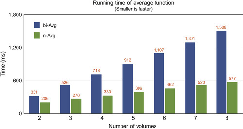
Based on the same strategy of n-ary operators, we propose a parallel efficient average function with hand-tuned performance for all number of inputs from 1 to 8, as illustrated in
Figure 48.3
.
 |
| Figure 48.3
n-ary average function versus binary average operator.
|
Gradient computation
is a frequently used and essential function in image processing. Based on the locality of the computation, several optimization techniques may be applied, such as 1-D linear texture cache, 3-D texture, or implicit cache through shared memory. Among these techniques, we found the 3-D stencil method
[11]
using the shared memory the most effective.
Table 48.1
shows the runtime comparison in milliseconds of different gradient computations: simple approach, linear 1-D texture, 3-D texture, and our shared-memory implementation.
| Gradient Method | Simple | 1-D Linear | 3-D Texture | Shared |
|---|---|---|---|---|
| 3.4 | 3.0 | 6.8 | 1.6 | |
| 9.5 | 8.9 | 21 | 5.2 |
The result shows that gradient computation on shared memory exploiting the 3-D stencil technique is twice as fast as using the linear texture cache.
48.3.3. ODE Integration
The ODE integration computes the deformation field by integrating velocity along the evolution path. A computationally efficient version of ODE integration is the recursive equation that computes the deformation at time
 based on the deformation at time
 ; that is,
 . This computation could be done by the reverse mapping operator (Figure 48.4
), which assigns each destination grid point a 3-D interpolation value from the grid neighbor points in the source volume. Fortunately, on GPUs, this interpolation process is fully hardware accelerated with 3-D texture volume support from CUDA 2.0 APIs. This optimization greatly reduces the computational cost of the ODE integration.
. This computation could be done by the reverse mapping operator (Figure 48.4
), which assigns each destination grid point a 3-D interpolation value from the grid neighbor points in the source volume. Fortunately, on GPUs, this interpolation process is fully hardware accelerated with 3-D texture volume support from CUDA 2.0 APIs. This optimization greatly reduces the computational cost of the ODE integration.
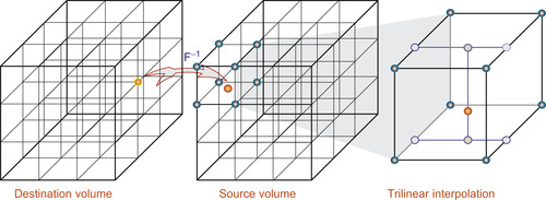 |
| Figure 48.4
Reverse mapping based on 3-D trilinear interpolation.
|
As shown in
Algorithm 2
, optimal velocity is computed from the force function by solving the Navier-Stokes equation
 Often
Often
 is negligible, and
Equation 48.2
simplifies to the Helmholtz equation
is negligible, and
Equation 48.2
simplifies to the Helmholtz equation
 where
where
 and
and
 are generally used in practice. Note that there is no crossing term in the Helmholtz equation; that means the solver could independently run on each dimension.
(48.2)
(48.3)
Although the ODE computation can be easily optimized simply by utilizing the 3-D hardware interpolation, the PDE solver is less amenable to GPU implementation. The PDE is a sparse linear system with size
 , where
 is the volume of the input. A direct dense linear package such as CUDA BLAS cannot handle the problem. What we need is a sparse solver. There are many different methods to solve a sparse linear system. The two most common and efficient ways are explicit solvers in the Fourier domain and implicit solvers using iterative refinement methods such as conjugate gradient (CG), successive over relaxation (SOR), or multigrid.
In our framework we support different methods such as FFT, SOR, and CG. There are multiple reasons to support multiple techniques, rather than a single method. Although the FFT solver is the slowest, it produces an exact PDE solution. Although the others are significantly faster, they produce only approximate solutions, which often have local smoothing effects. The inability to account for the influence of spatially distant data points in the initial solution slows down the convergence rate of these methods in the long run. Consequently, they require more iterations to achieve the same result as the FFT approach. Because of smoothing properties of the velocity field, the variance in the solution of the PDE solver between two successive steps is often small. This variance can be captured adequately by the iterative solvers in a few iterations. This is made possible by using the previous solution as an initial guess for the iterative solver in the next step. For the first iteration, without a proper guess, iterative solvers are often slow to converge, so they require a large number of iterations and may quickly become slower than the FFT approach. Therefore, we use an FFT solver in the first iteration and then switch to iterative methods. Our experiments show that the hybrid CG solver that starts with an FFT step produces exactly the same results as an FFT method, but is almost three times faster.
For the details on the FFT solvers we refer the reader to
[12]
. Here, we will discuss the implementation of SOR and CG methods.
48.3.5. Successive Over Relaxation Method
The successive over-relaxation (SOR) is an iterative algorithm proposed by Young for solving a linear system
[13]
. Theoretically, the 3-D FFT solver has a complexity of
 versus
 for SOR. However, the complexity analysis does not account for the fact that SOR is an iterative refinement method whose convergence speed largely depends on the initial guess. With a close approximation of the result as the initial value, it normally requires only a few iterations to converge. The same argument is true for other iterative methods such as CG.
We observe that in the elastic deformable framework with steady fluids, the changes in the velocity field are quite small between greedy steps. The computed velocity field of the previous step is inherently
a good approximation for the current one. In practice, we typically need 50 to 100 SOR iterations for the first greedy step, but only four to six iterations for each subsequent step.
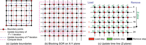
Our framework provides an SOR implementation with red-black ordering, as shown in
Figure 48.5
. This strategy allows for efficient parallelism because we update only points of the same color based on their neighbors, which have a different color. Also, red-black decoupling is proved to have a well-behaved convergence rate with the optimal over-relaxation factor
 defined in 3-D as
 .
.
 |
| Figure 48.5
Parallel block SOR; we assign each CUDA thread block a block of data to compute the black points inside the boundary shown by, and use that result to compute the point inside the boundary shown by. Two neighboring compute blocks share a four-grid-point-wide region.
|
We incorporate optimization techniques from the 3-D stencil buffer problem to exploit the fast shared memory available in CUDA and improve the register utilization of the algorithm (Algorithm 3
). We further improve the performance by increasing the arithmetic intensity of the data. This is done with merging steps of SOR that combines red-update steps and black-update steps of traditional SOR in one execution kernel. We also proposed
block-SOR
algorithms that we divide input volume into blocks, each fitting onto one CUDA execution block. We then exploit the shared memory to perform the merging step locally on the block. For simplicity, we illustrate the idea in 2-D in
Figure 48.5
, but it is generalized to arbitrary dimensions.
As shown in
Figure 48.5
the updated volume is two cells smaller in each dimension than the input. This reduction in size explains why we cannot merge an arbitrary number of steps in one kernel. To update the whole volume, we allow data overlaps among processing blocks, as shown in
Figure 48.5(b)
. Here, we allow data redundancy to increase memory usage. The configuration shown in
Figure 48.5(b)
, having a four-point-wide boundary overlap, is able to update one red-black merging step over a
 block using
 input. Likewise, a
 -merging step needs a data block of size
 . To quantify the benefit of SOR merging steps, we compute a trade-off factor
 such that:
 In 3-D, to update the volume block
 , we need
 volume inputs; the trade-off factor is
 . Note that the size of shared memory constraints the block size
 and merging level
 . In practice, we see benefits only if we merge one black and red update step per kernel call.
(48.4)
1:
Input
: Old velocity field
 and new force function

2:
Output
: Compute new velocity field

3: Allocate 4 shared mem arrays
 ,
,
 ,
,
 ,
,
 to store 4 slices of data
4: Load
 of 3-first slices to the registers of current thread
5: Load
 of 3-first slices to registers and shared memory
6: The boundary thread load the padding data of

7: Update the black point of the second slice

8:
for
 to
to
 do
{loop over Z direction}
do
{loop over Z direction}
9:
Load the
 and
and
 of the next slice to the free shared-mem array

10:
Update the black points of the
 slice
slice
11:
Update the red points of the
 slice
slice
12:
Write the
 to the global output,
 buffer is free to load the next slice
13:
Shift the value of
 and
and
 in the registers,
 ,
,
 ,
,

14:
Circular shift the shared memory array pointers,
 becomes

15:
end for
16: Update the red points on the last slice close to boundary
17: Write out the last slice
Algorithm 3
shows the pseudocode of our block-SOR implementation on CUDA. We further leverage the trade-off by limiting block-SOR in the 2-D plane only and exploit the coherence between consecutive layers in the third dimension to minimize data redundancy. On the Tesla, our block-SOR implementation using shared memory is two times faster than an equivalent version using 1-D texture cache.
Figure 48.5(c)
shows the updating time line in Z-dimension; it is clear that each node is computed by its neighbors, which are updated in previous steps.
48.3.6. Conjugate Gradient Method
Although the SOR method is specialized for solving PDEs on a regular grid, in practice the conjugate gradient approach is often the preferred technique because of several advantages:
• It is capable of solving a PDE on an irregular grid as well.
• It is simple to implement because it is built on top of basic linear operations.
• In general, it converges faster than the SOR method.
As shown in
Figure 48.7
, the CG algorithm is implemented in our framework as a template class with
 being the matrix presentation of the system. The only function required from
 is a matrix vector multiplication. The template allows for the integration of any sparse matrix vector multiplication package using an explicit presentation such as ELL, ELL/COO
[2]
and CRS
[1]
, or an implicit presentation that encodes the system matrix with constant values in the kernel.
is a matrix vector multiplication. The template allows for the integration of any sparse matrix vector multiplication package using an explicit presentation such as ELL, ELL/COO
[2]
and CRS
[1]
, or an implicit presentation that encodes the system matrix with constant values in the kernel.
Figure 48.6
is the implementation of the implicit matrix vector multiplication with Helmholtz Matrix and zero-boundary condition. The texture cache is used to access neighboring information to
achieve maximal memory bandwidth. Our experiments showed that in the case of the regular grid, the implicit approach allows for a more efficient matrix vector multiplication because the matrix does not consume memory bandwidth. As shown in
Table 48.2
, it is up to 2.5 times faster than explicit implementations
[2]
. The performance is measured in GFLOPs with Helmholtz Matrix vector multiplication.
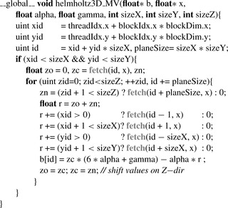 |
| Figure 48.6
Matrix vector multiplication CUDA kernel with implicit Helmholtz Matrix.
|
 |
| Figure 48.7
CG solver template.
|
| Matrix size | 64 3 | 96 3 | 128 3 | 160 3 | 192 3 | 224 3 | 256 3 |
| Implicit | 17 | 37 | 53 | 42 | 54 | 51 | 59 |
| Explicit Dia | 25 | 27 | 27 | 25 | 25 | 25 | 27 |
| Explicit Ell | 16 | 17 | 17 | 16 | 16 | 16 | 16 |
1:
Input
:
N
volume inputs, multi-scale information
2:
Output
: Template atlas volume
3:
for all
 to
to
 {loop over the scales}
4:
Read
 ,
,
 , fluid registration parameters at the scale
5:
for
 to
to
 {loop over the images}
6:
if
 then
{first level scale - original image}
then
{first level scale - original image}
7:

8:
else
{down sample the image}
9:
Blur the image
10:
Down sample
11:
end if
12:
if
 then
{first iteration}
then
{first iteration}
13:
 ,
,

14:
Copy the sample image

15:
else
16:
Up sample deformation field
17:
Up sample velocity field
 {if needed}
18:
Update deformed image

19:
end if
20:
end for
21:
Apply the atlas construction procedure at this scale
22:
end for
The concept of our multiscale framework is derived from the multigrid technique, which computes an approximate solution on a coarse grid and then interpolates the result onto the finer grid. As the solution on the coarse grid generates a good initial guess of solution on the finer grid, it speeds up the convergence on the finer level. In addition to reducing the number of iterations, multiresolution increases the robustness with respect to noise in the input data because it is capable of handling local optimums inherent to gradient-descent optimization. We design a multiscale GPU interface (Algorithm 4) based on two main components: the downscale Gaussian filter and the upscale sampler.
The downscaled filter is composed of a low-pass filter followed by a down sampler. The low-pass filter is a 3-D-Gaussian filter that is implemented using 1-D-Gaussian separable filters along each axis. We discovered that it is more efficient to implement this 3-D filter based on the separable-recursive Gaussian filter, rather than convolution-based or FFT-based approaches. Our recursive version is generalized from the 1-D recursive version (see NVIDIA SDK
RecursiveGaussian
) with a circular-dimension shifting 3-D transpose. As shown in
Table 48.3
the 3-D recursive version is the fastest, and its runtime, measured in milliseconds, is independent of the kernel size. The other methods in comparison are: a separable filter, a circular-dimension shifting combined with the 1-D filter in the fastest dimension, and an FFT-based filter.
While the down sampler simply fetches values from the grid, the up sampler is the reverse-mapping operation from the grid point of the finer scale to the point value of the coarser grid based on the trilinear interpolation. Here, we used the same optimization as for the ODE integration.
Our multiresolution framework can be employed in any 3-D image-processing problem to improve both performance and robustness.
48.3.8. Multi-GPU Processing Model
Computing systems in practice have to deal with a large amount of data that cannot be processed directly and efficiently by a single-processing system. GPUs are no exception to this limitation. Hence, the development of a parallel multi-GPU framework is necessary, especially for exploiting the total power of multi-GPU systems (multi-GPU desktops) or GPU cluster systems.
In the following, we address the two main bottlenecks of multi-GPUs and cluster implementations: the limited CPU-GPU bandwidth, which is about 20 times slower than the local GPU memory bandwidth, and the limited network bandwidth between compute nodes, which is an order of magnitude slower than CPU-GPU bandwidth. Our computational model aims at minimizing the amount of data transfer over the slow media, exploiting existing APIs such as MPI, and moving most of the computation from the CPUs to the massively parallel GPUs.
Multi-GPU Model
We first proposed a multiple-input multi-GPU model
[7]
. The key idea was to maximize the total volume of inputs that the system can handle. In other words, by maximizing the number of inputs per node, we increase the
arithmetic intensity
of each processing node.
We divide the inputs between GPU nodes and assign a GPU memory buffer at each node to serve both as an accumulation buffer and an average input buffer. The output buffer is used to sum up the local deformed volumes; the input buffer contains the new average and is shared among volumes of the node.
At each iteration, we compute the local accumulation buffers and send the result to the server to compute the global accumulation buffer. The new aggregate volume is read back to GPU nodes. Next, we perform a volume division on the GPUs to update the average.
Our aggregate model is more efficient than our previous average model
[7]
because it yields the same memory bandwidth, but moves the computation from CPUs to GPUs; hence, it is able to exploit the computational power of the GPU. This strategy minimizes both the overall cost per volume element as well as the data transfer over the low-bandwidth channel.
GPU Cluster Model
We generalize the multiple-input multi-GPU model to a higher level to build a computationally efficient framework on GPU clusters. As displayed in
Figure 48.8
, we maintain two buffers on a CPU-multi-GPU processing node: an output accumulation buffer and an input aggregate buffer that is shared among the members of the buffer's GPUs. These two CPU memory buffers are used as the interface memory to other processing nodes through the MPIs. As we used the aggregated model instead of the average, we can directly exploit the MPI all-reduce function to efficiently compute and update the accumulated volume to all processing nodes. Next, we address the load distribution problem of the GPU cluster implementation.
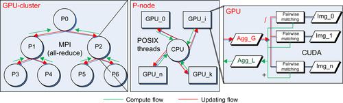 |
| Figure 48.8
Multi-GPU framework on the GPU cluster.
|
Load Balancing
We consider load balancing on a system with homogeneous GPUs with
 ,
,
 ,
,
 being the number of inputs, GPUs, and CPUs. Our test system is a Tesla S1070 cluster, with each node having dual-GPUs, thereby implying that
 .
.
On the cluster, the total runtime per iteration is computed by
 . As the number of GPUs per node is fixed,
 — the amount of time to compute the aggregate among GPUs of the same node — is fixed. Consequently, we must reduce
 and/or
 to improve the runtime.
First, we assume that
 is fixed, then
 — the amount of time to accumulate and distribute the result between CPUs — is defined.
 depends on the maximum number of inputs per GPU, which is at least
 . This number is optimal if inputs are distributed evenly between GPUs, not CPUs because CPUs may have a variable number of GPUs attached. So our first strategy is distributing
inputs evenly among GPU nodes. With this strategy, there is at most one unbalanced GPU, and the GPU runtime with synchronization is optimal.
. This number is optimal if inputs are distributed evenly between GPUs, not CPUs because CPUs may have a variable number of GPUs attached. So our first strategy is distributing
inputs evenly among GPU nodes. With this strategy, there is at most one unbalanced GPU, and the GPU runtime with synchronization is optimal.
Second, it is highly likely that the MPI all-reduce function performs the binary tree down-sweep to accumulate the volume and binary tree up-sweep to distribute the sum to all nodes, as shown in
Figure 48.8
. This yields a minimal amount of data transferred over the network, that is,
 . It is suggested that the amount of data transfer over the network increases linearly with the number of CPU nodes, and therefore, fewer CPUs implies smaller delay. This hypothesis is confirmed in our cluster in the experiment (see
Figure 48.9
).
. It is suggested that the amount of data transfer over the network increases linearly with the number of CPU nodes, and therefore, fewer CPUs implies smaller delay. This hypothesis is confirmed in our cluster in the experiment (see
Figure 48.9
).
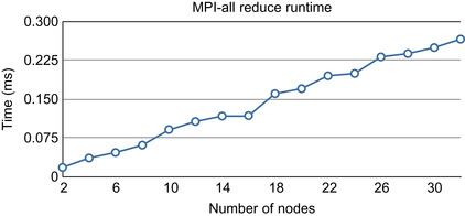 |
| Figure 48.9
MPI-all reduce runtime on an infiniband network with OpenMPI 1.3 shows a linear dependency on the number of nodes.
|
To reduce the number of CPU nodes, we increase the GPU workload. Note that from the first strategy we want to increase all GPUs with the same number of volumes so that the computation is balanced. Let us increase this number by one; the total runtime then is
 where
where
 is the number of GPUs reduced by increasing the workload. This equation gives us an approximation of running time as the number of volumes per GPU changes. Hence, we can vary the capability on the GPU node to achieve a better configuration. Note that in the dual-GPU system, if the number of volumes per GPU is less than
 , when we increase the number of volumes per GPU by one, we can decrease the number of CPUs at least by two.
Our load-balancing strategy is as follows: First, the users choose the number of nodes. Based on this choice the system computes the number of inputs per GPU. The components’ runtime is then determined with a one-iteration dry run on the zero-initialized volumes that require no data from the host. Next, the optimizer varies the number of volumes per GPU, recomputes the number of CPU nodes, and computes the total runtime. This heuristic yields an optimal configuration to handle the problem.
48.3.9. Performance Tuning
To further improve the performance, we now present a volume-clipping optimization and the scratch memory model. Those techniques are specially applied for multi-image-processing problems.
Volume clipping is the final step of the preprocessing, which includes
• Rigid alignment and affine registration
• Intensity calibration and normalization
• Volume clipping
The rigid alignment and affine registration guarantee all inputs to be in the same space, while the preprocessing distances between them are minimal. This strategy significantly speeds up the convergence of the image registration process. The intensity calibration ensures that the intensity range of the inputs are matched and are normalized for visualization purposes. Although these two preprocessing steps are generally applied in a regular image registration framework, the volume clipping is a special optimization scheme applied for the brain image to reduce processing time.
Pointwise computations on zero-data usually return zero; we call this data redundant. This redundancy happens near the boundary of the volume. The volume-clipping strategy first computes the nonzero data-bounding boxes and then tightly clips all the volumes to the common bounding box with guarded boundary conditions. In practice, the volume of clipping inputs can be significantly smaller than a typical input volume; for example, the
 brain images in our experiment have a common volume of size
 , a volume ratio of three. Because the runtime of a function is proportional to the volume of the inputs, we experienced three to four times speedup just by applying this volume-clipping strategy. Note that this optimization is more effective at PDE SOR solvers than FFT-based solvers because the latter require a power of two volume size to be computationally efficient.
Scratch Memory Model
It is always a challenge to implement 3-D processing frameworks on GPUs as the parallel processing scheme often requires more memory than it would on CPUs. To deal with this memory problem, we proposed a scratch memory model, a shared-temporary memory space, coupled with different optimization techniques including:
Zero-copy operation based on pointer swapping to reduce the redundant memory copy from scratch memory (Figure 10(a)
)
A circular buffer technique to reduce memory copy redundancy and also memory storage requirements for computation in a loop (Figure 10(b)
)
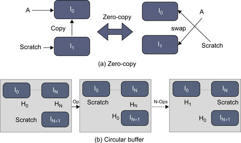 |
| Figure 48.10
Optimization strategies with the scratch memory model.
|
The use of the scratch memory model helps us to significantly reduce the memory requirement. In particular, in the case of the greedy iterative atlas construction, we only need a single image buffer and two 3-D-vector buffers for an arbitrary number of inputs on a single GPU device. Consequently, we are able to process 20 brain volumes with 4GB global memory, or 40 brain volumes on a single dual-GPU node.
48.4. Final Evaluation and Validation of Results, Total Benefits, and Limitations
The system we used in our experiment is a 64-node Tesla S1070 cluster, each containing two GPUs. Communication from the host to GPU was via the external x16 PCIe bus, and inter-node
communication was implemented through a 20 Gb 4x DDR infiniband interconnect. The program was compiled with CUDA NVCC 2.3. For multiresolution, we performed a two-scale computation with 25 iterations in the coarse level and, 50 iterations in the finer level, with parameters set
 ,
,
 , and
, and
 . The three solvers used in the comparison were FFT solver, the block-SOR, and conjugate gradient(CG). The runtime did not include the data-loading time that depends on the hard disk system.
48.4.1. Quality Improvements
To evaluate the robustness and stability of the atlases, we use the random permutation test proposed by Lorenzen
et al.
[10]
. The method is capable of estimating the minimum number of inputs required to construct a stable atlas by analyzing mean entropy and the variance of the average template. We generated 13 atlas cohorts,
 , each including 100 atlases constructed from
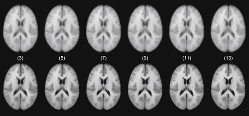
 input images chosen randomly from the original dataset. The 2-D mid-axial slices of the atlases are shown in
Figure 48.11
. The normal average atlases are blurry, and ghosting is evident around the lateral ventricles, as well as near the boundary of the brain. In this case, the greedy iterative average template appears to be much sharper, preserving anatomical structures.
input images chosen randomly from the original dataset. The 2-D mid-axial slices of the atlases are shown in
Figure 48.11
. The normal average atlases are blurry, and ghosting is evident around the lateral ventricles, as well as near the boundary of the brain. In this case, the greedy iterative average template appears to be much sharper, preserving anatomical structures.
 |
| Figure 48.11
Atlas results with 3, 5, 7, 9, 11, and 13 inputs constructed by arithmetically averaging rigidly aligned images (top row) and greedy iterative average template construction (bottom row).
|
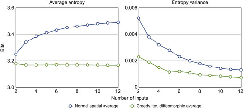
The quality of the atlas construction is visibly better than the least MSE normal average. The entropy results shown in
Figure 48.12
also confirm the stability of our implementation. As the number of inputs increases, the average atlas entropy of the simple averaging intensity increases, while the greedy iterative average template decreases owing to much higher individual sharpness. This quantitatively asserts the visible quality improvement in
Figure 48.11
. The atlases become more stable with respect to the entropy as the standard deviation decreases with an increasing number of inputs. After cohort
 , the atlas entropy mean appears to converge. So we need at least eight images to create a stable atlas representing neuroanatomy.
 |
| Figure 48.12
Mean entropy and variance of atlases constructed by arithmetically averaging and the greedy iterative average template.
|
We compare the speedup of the multiscale framework to the single-scale version with a pairwise matching problem to produce comparable results. Experiments show that we generally need 25 iterations in
the second level and 50 iterations in the first level to produce similar results, whereas we need 200 iterations with a single-scale implementation. The speedup factor is about 3.5 and comes primarily from lowering the number of iterations in the finest level.
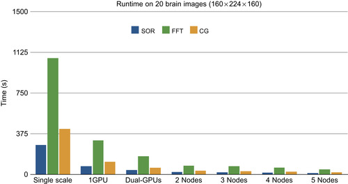
We quantify the compute capability and scalability of our system in two cases. First, by applying the scratch memory technique, we are able to handle 20 T1 images of size
 on a single GPU device. We measure the performance with one GPU device (multiscale), one single node with dual-GPUs (multiscale multi-GPUs), and two, four, and five GPU nodes (multiscale cluster) in reference to a single-scale version on the 20-brain input set. As shown in
Figure 48.13
the multiscale version is about 3.5 times faster than the single-scale version, whereas our multi-GPU version is twice as fast as a single device. The cluster version shows a linear performance improvement to the number of nodes.
on a single GPU device. We measure the performance with one GPU device (multiscale), one single node with dual-GPUs (multiscale multi-GPUs), and two, four, and five GPU nodes (multiscale cluster) in reference to a single-scale version on the 20-brain input set. As shown in
Figure 48.13
the multiscale version is about 3.5 times faster than the single-scale version, whereas our multi-GPU version is twice as fast as a single device. The cluster version shows a linear performance improvement to the number of nodes.
 |
| Figure 48.13
Runtime to compute the average atlas of the 20 T1 brain images (144 × 192 × 160) with multiscale and/or multi-GPUs, cluster implementation in reference to one-scale version.
|
Second, we experiment with the full dataset of 315 volumes of T1 input size 144 × 192 × 160. For the first time we handle the whole dataset on eight nodes of the GPU cluster. We measure the performance with 8, 12, 16, 20, 24, 28, and 32 nodes. On the 32-core Intel Xeon server X7350, 2.93 GHz with 196 GB of shared memory, which is able to load the whole dataset in the core, the CPU-optimized greedy implementation took 2 minutes for a single iteration. As shown on
Figure 48.14
, it only takes the SOR solver about 70 seconds to compute the average on eight nodes of the GPU cluster and only 20 seconds on 32 nodes, which is two orders of magnitude faster than the 32-core CPU server.
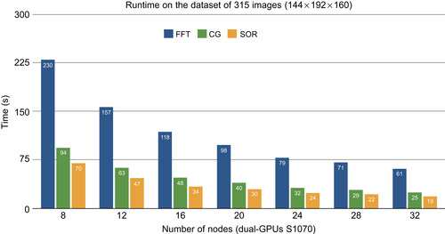 |
| Figure 48.14
Multiscale runtime to compute the average atlas of the 315 T1 brain images (144 × 192 × 160) with different PDE solver.
|
48.5. Future Directions
In this chapter we have presented our implementation of the unbiased greedy iterative atlas construction on multi-GPUs; however, this is only a showcase to illustrate the computing power and efficiency of our
processing framework. As we mentioned in the introduction, the atlas construction problem is a basic foundation for a class of diffeomorphic registration problems to study the intrapopulation variability and interpopulation differences. The ability to produce the result in real time enables us to understand the research influence of this powerful technique. Also the framework allows us to implement more sophisticated registration problems, such as LDDMM, metamorphosis, or image current. Although each technique has a different trade-off between quality of results and the computation involved, our framework is capable of quantifying those trade-offs to suggest a good solution for the practical problem suitable with inputs and the accessible computational power.
Although the system has the capability to handle large amounts of data, it requires a single matching pair to be completely solvable on a single-GPU node; however, such compute power is not always available. So we are considering extending the processing power of a single-GPU system using an out-of-core technique. This requires a major redesign of our system; however, it is a required feature of our processing system to handle the ever-growing amounts of data in the future.
Note that our code is a part of the AtlasWerks project, which is free for research purposes and is available to download at
http://www.sci.utah.edu/software.html
.
Acknowledgments
This research has been funded by the National Science Foundation grant CNS-0751152 and National Institute of Health Grants R01EB007688 and P41-RR023953. L. Ha was partially supported by the Vietnam Education Foundation fellowship. Specially, the authors thank Sam Preston, Marcel Prastawa, and Thomas Fogal for their time and feedback on the work.
[1]
M.M. Baskaranm, R. Bordawekar, Optimizing sparse matrix-vector multiplication on GPUs, IBM Technical Report, 2008. Available from:
http://domino.watson.ibm.com
.
[2]
N. Bell, M. Garland,
Implementing sparse matrix-vector multiplication on throughput-oriented processors
,
In:
SC ’09: Proceedings of the Conference on High Performance Computing Networking, Storage and Analysis, 2009
Portland, Oregon, ACM, New York
. (2009
), pp.
1
–
11
.
[3]
M. Bro-Nielsen, C. Gramkow,
Fast fluid registration of medical images
,
In:
VBC ’96: Proceedings of the 4th International Conference on Visualization in Biomedical Computing, 1996
(1996
)
Springer-Verlag
,
London, UK
, pp.
267
–
276
.
[4]
G.E. Christensen, M.I. Miller, M.W. Vannier, U. Grenander,
Individualizing neuroanatomical atlases using a massively parallel computer
,
Computer
29
(1996
)
32
–
38
.
[5]
G.E. Christensen, R.D. Rabbitt, M.I. Miller,
Deformable templates using large deformation kinematics
,
Image Proc. IEEE Trans. Image Proc.
5
(10
) (1996
)
1435
–
1447
.
[6]
B.C. Davis, P.T. Fletcher, E. Bullitt, S. Joshi,
Population shape regression from random design data
,
In:
Proceeding of the 11th IEEE International Conference on Computer Vision (ICCV 2007)
(2007
), pp.
1
–
7
.
[7]
L.K. Ha, J. Krüger, P.T. Fletcher, S. Joshi, C.T. Silva,
Fast parallel unbiased diffeomorphic atlas construction on multi-graphics processing units
,
In:
EUROGRAPHICS Symposium on Parallel Graphics and Visualization
(2009
)
;
Available from:
http://www.sci.utah.edu/~csilva/papers/egpgv2009.pdf
.
[8]
J. Hoberock, N. Bell,
Thrust: A Parallel Template Library, Version 1.3
(2009
)
;
Available from:
https://www.ohloh.net/p/thrust
.
[9]
S. Joshi, B. Davis, M. Jomier, G. Gerig,
Unbiased diffeomorphic atlas construction for computational anatomy, neuroimage
23
(Suppl.
) (2004
)
S151
–
S160
.
[10]
P. Lorenzen, B. Davis, S. Joshi,
Unbiased atlas formation via large deformations metric mapping
,
In: (Editors: J.S. Duncan, G. Gerig)
Medical Image Computing and Computer Assisted Intervention (MICCAI)
Int. Conf. Med. Image Comput. Comput. Assist. Interv. (MICCAI)
,
vol. 8 (Pt. 2)
(2005
), pp.
411
–
418
.
[11]
P. Micikevicius,
3D finite difference computation on GPUs using CUDA
,
In:
Proceedings of 2nd Workshop on General Purpose Processing on Graphics Processing Units, GPGPU2, 2009
New York
. (2009
), pp.
79
–
84
.
[12]
NVIDIA, CUDA Technical Training, Technical report, NVIDIA Corporation, 2009.
[13]
D. Young,
Iterative Solution of Large Linear Systems
. (1997
)
Academic Press
.
..................Content has been hidden....................
You can't read the all page of ebook, please click here login for view all page.