
Chapter 49. GPU-Accelerated Brain Connectivity Reconstruction and Visualization in Large-Scale Electron Micrographs
Won-Ki Jeong, Hanspeter Pfister, Johanna Beyer and Markus Hadwiger
The reconstruction of neural connections to understand the function of the brain is an emerging and active research area in neuroscience. With the advent of high-resolution scanning technologies, such as 3-D light microscopy and electron microscopy (EM), reconstruction of complex 3-D neural circuits from large volumes of neural tissues has become feasible. Among them, only EM data can provide sufficient resolution to identify synapses and to resolve extremely narrow neural processes. Current EM technologies are able to attain resolutions of three to five nanometers per pixel in the x-y plane. Because of its extremely high resolution, an EM scan of a single section from a tiny brain tissue of only a half cubic millimeter in size can easily reach up to tens of gigabytes, and the total scan of the tissue sample can be as large as several hundred terabytes of raw data.
Figure 49.1
is an example of a high-resolution EM image in different zoom levels.
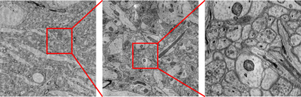 |
| Figure 49.1
An example of a high-resolution EM scan of a mouse brain. From left to right: A zoomed-out view of an EM image, 4 × magnification, and 16 × magnification. The pixel resolution of an EM image that we are dealing with is around three to five nanometers; this resolution allows scientists to look at nanoscale cell structures, such as synapses or narrow axons, as shown in the image on the right.
|
These high-resolution, large-scale datasets pose challenging problems, for example, how to process and manipulate large datasets to extract scientifically meaningful information using a compact representation in a reasonable processing time. Among all, reconstructing a wire diagram of neuronal connections in the brain is the most important challenge we tackle. In this chapter, we introduce a GPU-accelerated interactive, semiautomatic axon segmentation and visualization system
[1]
. There are two challenging problems we address: (1) interactive 3-D axon segmentation and (2) interactive 3-D image filtering and rendering of implicit surfaces. We exploit the high-throughput, massively parallel computing power of recent GPUs to make the proposed system run at interactive rates. The main focus of this chapter is introducing the GPU algorithms and their implementation details, which are the core components of our interactive segmentation and visualization system.
49.2. Core Methods
49.2.1. Semiautomatic Axon Segmentation
Axons are pathways that serve as a communication network to connect distant cell bodies, and are presented as thin, elongated tubes in 3-D space. Our approach
[1]
to extract such long and thin 3-D tubular structures is combining 2-D segmentation and 3-D tracking methods. Each 2-D segmentation is
done on a small 2-D region-of-interest (ROI) image sampled from the input 3-D volume. Therefore, it scales well to the large EM images we are acquiring. We use the active ribbon model
[10]
to segment the outer boundary of the axon membrane on each 2-D ROI. As each cell membrane is extracted, we trace the center of each axon cross-section using a forward Euler integration method to finally create a 3-D model of the axon.
Figure 49.2
(left) is a pictorial description of the active ribbon model, and (right) is a screenshot of our 3-D axon segmentation in action.
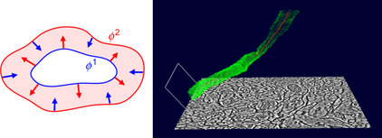 |
| Figure 49.2
3-D axon segmentation consists of 2-D cell membrane segmentation and 3-D tracking. Left: The active ribbon model. Right: 3-D tracking of an axon as a collection of 2-D ribbons.
|
The active ribbon model consists of two deformable interfaces,
 and
and
 in
Figure 49.2
(left), that push or pull against each other until they converge to the inner and outer wall of the cell membrane. The deformable model we employed is a multiphase level set
[11]
, where the Ω-level set is a set of points whose distance is
in
Figure 49.2
(left), that push or pull against each other until they converge to the inner and outer wall of the cell membrane. The deformable model we employed is a multiphase level set
[11]
, where the Ω-level set is a set of points whose distance is
 . We use two level sets whose partial differential equations (PDE) are defined by various internal and external forces to enhance the smoothness of the interfaces and to preserve the band topology as follows:
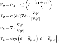
 where
where
 is the data-dependent speed to move the interface toward the membrane,
 is the ribbon consistency speed to keep the distance between two level sets constant,
 is the mean curvature speed
to maintain the shape of the interface as smooth as possible, and
is the mean curvature speed
to maintain the shape of the interface as smooth as possible, and
 is the image correspondence speed to enforce the level sets to transfer from one slice to the next correctly.
(49.1)
Solutions to
Equation 49.1
can be computed using an iterative update scheme. To keep the topology of the active ribbon consistent during the level set iteration, we need to evaluate the distance between the two zero level sets. Because the active ribbon does not guarantee the correct distance after deformation owing to the combination of various force fields, we need to correct the error by computing the signed distances from the level sets after the level set equation update. We also include an image correspondence force into the level set formulation to robustly initialize the location of the interfaces on subsequent slices. The computational challenges we address are
• Multiphase level set computation;
• Re-initialization of level sets using distance transform; and
• Image correspondence computation using nonrigid image registration.
We implemented those time-consuming numerical methods on the GPU to achieve interactive performance.
Solving PDEs using an iterative solver on parallel systems is a well-studied problem
[3]
. However, mapping it on massively parallel architectures, such as GPUs, has been attempted only recently
[4]
. Although many iterative solvers are based on global update schemes (e.g., the Jacobi update), the most efficient approach to solve the level set PDE is using adaptive updating schemes and data structures, such as narrow band
[9]
or sparse field
[12]
approaches. Such adaptive schemes are typically not good candidates for parallelization on the GPU, but we overcome the problem by employing data structures and algorithms that exhibit spatially coherent memory access and temporally coherent executions. Our approach is using a
block-based
data structure and update scheme as introduced in
[1]
[2]
and
[4]
. The input domain is divided into blocks of predefined size, and only the blocks containing the zero level set, that is, the
active blocks
, will be updated. Entire data points (or nodes) in a block are updated concurrently using parallel threads on the GPU. This parallel algorithm can be used to update level set PDEs and to compute distance transforms.
On the other hand, the GPU nonrigid image registration that we implemented is a standard global energy minimization process using the Jacobi update, which is a gradient descent method implemented on the GPU. The energy function we minimize is:
 where
where
 and
and
 are two input images, Ω is the image domain,
 is the image
 deformed by the vector field
 , and
, and
 is a regularization parameter. The solution vector field
 that minimizes
Equation 49.2
gives pixel-to-pixel correspondence between
that minimizes
Equation 49.2
gives pixel-to-pixel correspondence between
 and
and
 . In order to find
 , we use a gradient flow method along the negative gradient direction of
 with respect to
 .
.
(49.2)
49.2.2. 3-D Volume and Axon Surface Visualization
For the visualization of the high-resolution and extremely dense and heavily textured EM data, we support the inspection of data prior to segmentation, as well as the display of the ongoing and the final segmentation.
To visualize the complex structure of interconnected nerve cells and to highlight regions of interest (e.g., myelinated axons) prior to segmentation, we have implemented on-the-fly nonlinear noise removal and boundary enhancement (Figure 49.3(a)
). To display the ongoing and final neural process segmentation, we combine direct volume rendering with implicit surface ray casting in a single rendering pass (Figure 49.3(b)
).
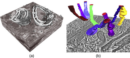 |
| Figure 49.3
Volume rendering of electron microscopy (EM) data to depict neural processes. (a) On-the-fly boundary enhancement. (b) 3-D visualization of segmented neural processes embedded in the volume.
|
Our visualization approach is built upon a GPU-based raycaster
[8]
that supports bricking for handling of large datasets.
Bricking
is the process of splitting up a single volume into several individual volume bricks. Bricking by itself does not reduce overall memory consumption; however, it can reduce memory consumption on the GPU by downloading only currently active bricks (i.e., the current working set of bricks) to GPU memory.
On-Demand Volume Filtering Using the GPU
To improve the visual quality of the volume rendered EM data and to highlight regions of interest prior to segmentation, we have implemented on-the-fly nonlinear noise removal and boundary enhancement filters. A local histogram-based boundary metric
[5]
is calculated on demand for currently visible parts of the volume and cached for later reuse. During ray casting we use the computed boundary values to modulate the current sample's opacity with different user-selectable opacity weighting modes (e.g., min, max, alpha blending), thereby enhancing important structures like myelinated axons, while fading out less important regions. For noise removal, we have implemented Gaussian, mean, median, bilateral, and anisotropic diffusion filters in both 2-D and 3-D with variable neighborhood sizes.
We have implemented a general on-demand volume-filtering framework entirely on the GPU using CUDA, which allows for changing filters and filter parameters on the fly, while avoiding additional disk storage and bandwidth bottlenecks for terabyte-sized volume data.
Filtering is performed only on currently visible 3-D bricks of the volume, depending on the current viewpoint, and the computed bricks are stored directly on the GPU, using a GPU caching scheme. This avoids costly transfers to and from GPU memory, while at the same time, avoiding repetitive recalculation of already filtered bricks. During visualization, we display either the original volume, the de-noised volume, the computed boundary values, or a combination of the above.
For visualizing segmented neural processes in 3-D, we depict the original volume data together with semitransparent iso-surfaces that delineate segmented structures such as axons or dendrites in a single front-to-back ray casting step implemented in CUDA
[1]
.
Keeping our large dataset sizes in mind, we store the segmentation results in a very compact format, where each axon is represented as a simple list of elliptical cross sections. For an ongoing segmentation, the list of elliptical cross sections is continuously updated. For rendering, we use standard front-to-back ray casting with the addition of interpolating implicit surfaces from the set of ellipses on the fly. If, during ray casting, a sample intersects an implicit surface, the color and opacity of the surface are composited with the previously accumulated volume rendered part, and volume rendering is continued behind the surface. Therefore, during ray casting, we need to compute the intersections of rays with the implicit surface. The implicit surface itself is interpolated between two successive elliptical cross sections, which enclose the given sample position on a ray. We efficiently combine direct volume rendering with iso-surface ray casting
[8]
, using a single ray-casting CUDA kernel.
49.3. Implementation
We implemented the most time-consuming and computationally expensive components in our system using NVIDIA CUDA and have tested our implementation on NVIDIA GPUs.
49.3.1. GPU Active Ribbon Segmentation
Our GPU active ribbon segmentation consists of two parts: GPU level set update and GPU distance computation. GPU level set update is an inner loop of the main iteration and is iterated multiple times before the re-distance step corrects the errors incurred by the level set update. The entire process is depicted in
Figure 49.4
.
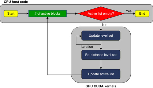 |
| Figure 49.4
A flowchart of the GPU active ribbon segmentation process.
|
Level Set Updating Using the GPU
Our GPU multiphase level set method manages two sets of signed distance fields, one for each active ribbon boundary, and updates each level set concurrently in order to preserve the topology of the active ribbon. Each individual level set is implemented using a streaming narrowband level set method
[4]
that updates the solution only in the active regions using a block-based GPU data structure. However, we do not explicitly check the boundary of each block for activation as in the original method. Instead, we simply collect all the blocks whose minimum distance to the zero level set is within the user-defined narrowband width. The distance to the zero level set is computed in the re-distance step, so we only need to find the minimum value per block using a parallel reduction scheme. In addition, each level set uses the other level set to update its value, so both level sets must be updated concurrently using the Jacobi update scheme and ping-pong rendering using extra buffers. Interblock communication across block boundaries is handled implicitly between each CUDA kernel call because the current level set values are written back to global memory at the end of each level set update iteration.
We efficiently manage the active list by storing and updating the entire list on the GPU, and only the minimum information is transferred to the CPU that is required to launch a CUDA kernel accordingly. The first element of the active list is the total number of active blocks, followed by a list of active
block indices. Therefore, the host code reads only the first element in the active list to launch a CUDA kernel with the grid size equal to the number of active blocks. To retrieve a correct block from global memory in the CUDA kernel code, we perform a one-level indirect access, i.e., reading an active block index from active list and computing the actual memory location of the block in global memory. The process is described in
Figure 49.5
. Updating the active list is performed in parallel on the GPU. If any pixel in the current block touches the narrowband, i.e., the minimum distance to the zero level set is smaller than the narrowband width, then the current block index is added to the active list in global memory. The active list is implemented as a preallocated 1-D integer array and an unsigned integer value that points to the last element in the array. To add a new active block index to the active list, we use
AtomicAdd()
to mutually exclusively access the last active list element index and increase it by one because many blocks can access it simultaneously.
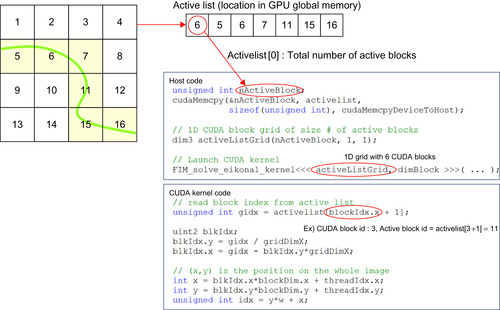 |
| Figure 49.5
An example of the host and CUDA kernel code showing how to use the active list. Six blocks among 16 blocks are active (left, colored in grey). The active list is stored in GPU global memory, and only the first element of the list (the total number of active blocks) will be copied to CPU memory. Then the host code launches the CUDA kernel with the 1-D grid size equal to the number of active blocks.
|
We implemented the level set solver using an explicit Euler integration scheme with a finite difference method. Because the curvature term in our level set formulation is a parabolic contribution to the equation, we use a central difference scheme for curvature-related computations; otherwise, an upwind scheme is used to compute first- and second-order derivatives
[9]
. Therefore, the update formula for
Equation 49.1
can be defined as follows:

 where
where
 and
and
 are the average pixel intensity of inner cell region and cell membrane, respectively,
 is the other level set in the active ribbon,
 is the function that returns a positive value if two level sets
 and
and
 are too close and a negative value otherwise,
 is the level set solution deformed by the vector field
 (in
Equation 49.2
) from the previous slice, and
(in
Equation 49.2
) from the previous slice, and
 and
and
 are approximated by the central difference and one-sided upwind difference scheme, respectively. Because pixel values are reused multiple times during derivative computation, we load the current block and its adjacent pixels into shared memory and reuse them to minimize global memory access.
Figure 49.6
shows the code snippet of the level set update code implemented in CUDA.
are approximated by the central difference and one-sided upwind difference scheme, respectively. Because pixel values are reused multiple times during derivative computation, we load the current block and its adjacent pixels into shared memory and reuse them to minimize global memory access.
Figure 49.6
shows the code snippet of the level set update code implemented in CUDA.
(49.3)
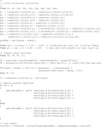 |
| Figure 49.6
A code snippet of the level set update code written in CUDA.
smem[]
is a float array allocated in shared memory that holds the current block and its neighboring pixels.
|
To quickly re-initialize the distance field using correct signed distance values after a number of level set updates, we employ a fast iterative method (FIM)
[2]
and solve the Eikonal equation on the GPU. The solution to the Eikonal equation gives the weighted distance to the source (seed) region. In our case we have a Euclidean distance because the speed value is one. We run the Eikonal solver four times, twice per level set, because the positive and negative distances from the zero level set should be computed independently. For example, to compute the positive distance, we set the distance value for all the pixels currently having negative values to zero. Those pixels are marked as source pixels and are treated as the boundary condition of the Eikonal equation.
FIM belongs to a class of label-correcting algorithms, which are well-known shortest path algorithms for graphs. Label-correcting algorithms do not use ordered data structures or special updating sequences that are common to label-setting algorithms such as the fast marching method
[9]
. Therefore, they map well to GPUs. FIM algorithms employ a list to simultaneously update multiple points in the active list using a Jacobi update step. To implement FIM on the GPU efficiently, we use a block-based data structure similar to our GPU level set implementation described in the previous section. Each active block is iteratively updated until it converges, and GPU threads update all the points in the same active block simultaneously. When an active block is converged, its neighboring blocks are checked, and any nonconvergent neighboring blocks are added to the active list. To check the convergence of a block we perform parallel reduction.
Algorithm 1
shows the pseudocode description of our GPU FIM, where
 represents a set of discrete solutions of the Eikonal equation,
 represents a
block of Godunov discretization of the Hamiltonian for a grid block
b
, and
represents a
block of Godunov discretization of the Hamiltonian for a grid block
b
, and
 (a grid of boolean values that is same size as
b
) and
(a grid of boolean values that is same size as
b
) and
 (a scalar boolean value) represent the convergence for nodes and a block
b
, respectively.
(a scalar boolean value) represent the convergence for nodes and a block
b
, respectively.

49.3.2. 3-D Axon Tracking Using Image Correspondence
We use an image registration method to compute slice-to-slice correspondence to robustly initialize the current level set using the previous segmentation result. We implemented a nonrigid (deformable) image registration method on the GPU that minimizes a regularized intensity-difference energy (Equation 49.2
). To compute the optimal
 that minimizes
 , we used a gradient flow method with discrete updates on
 along the negative gradient direction of
 . We implemented the gradient flow using semi-implicit discretization as a two-step iterative process as follows:

 where
where
 is a Gaussian kernel and
 is the convolution operator.
(49.4)
(49.5)
The first step, the iterative update process, is an explicit Euler integration method over time, and maps naturally to the GPU. Efficient GPU implementation of the iterative process is done using texture memory.
 and
and
 are the deformed image
 and gradient of
 by the vector field
 , respectively. Because of the regularization term in the energy function
 , the vector field
 smoothly varies from one point to another. Therefore,
 and
and
 are, in fact, spatially coherent random memory accesses, and this memory access pattern can benefit from using a hardware-managed texture cache and pixel interpolation. The second step, Gaussian convolution on the vector field
 , is implemented as consecutive 1-D Gaussian filtering along the x and y directions on a two-channel vector image
 .
.
49.3.3. GPU-Based Volume Brick Filtering Framework
Our on-demand volume-filtering algorithm for EM data works on a bricked volume representation and consists of several steps:
1. Detection of volume bricks that are visible from the current viewpoint
2. Generation of a list of bricks that need to be computed
3. Noise removal filtering for selected bricks, storing the results in the GPU cache
4. Calculation of histogram-based boundary metric on selected bricks, storing the results in the GPU cache
5. High-resolution ray casting with opacity modulation based on computed boundary values
To reduce communication between CPU and GPU, we perform all of the preceding steps on the GPU and only transfer the minimum information needed to launch a CUDA kernel back to the CPU.
To store bricks that have been computed on the fly we use a dynamic GPU caching scheme. Two caches are allocated directly on the GPU: one cache to store de-noised volume bricks and the second cache to store bricks containing the calculated boundary values. First, the visibility of all bricks is updated for the current viewpoint in a first ray casting pass and saved in a 3-D array corresponding to the number of bricks in the volume. Next, all bricks are flagged as either: visible/not visible and present/not present in cache. Visible bricks that are already in the cache do not need to be recomputed. Only visible bricks that are not present in the cache need to be processed. Therefore, the indices of
“visible, but not present” bricks are stored for later calculation. During filtering/boundary detection the computed bricks are stored in the corresponding cache. A small lookup table is maintained for mapping between brick storage space in the cache to actual volume bricks. Unused bricks are kept in the cache for later reuse. However, if cache memory gets low, unused bricks are flushed from the cache using an Lease-Recently-Used (LRU) scheme and replaced by currently visible bricks.
49.3.4. GPU Volume Brick Boundary Detection
As described in
Section 49.3.3
, for every view we determine a list of visible bricks in the volume during ray casting. We then perform filtering and boundary detection only for these visible bricks.
The boundary detection algorithm that we are using is based on the work of Martin
et al.
[5]
, which introduced a very robust method for detecting boundaries in 2-D images based on comparisons of local half-space histograms. In contrast to simpler edge detectors, this approach works very well in the presence of noise and can be used with arbitrary neighborhood sizes for computing the local histograms. For our EM data this boundary detection produces very good results, for example, in highlighting the boundaries of axons. The general idea is to go over all possible boundary directions for any given pixel, and compute a boundary value for each of the directions. The boundary value corresponds to the strength or probability of there being a boundary across the tested direction. The boundary value is computed by comparing the local histogram of the neighborhood on one side of the boundary with the local histogram of the neighborhood on the other side. The boundary in a given direction is strong when the two histograms are very different and weak when the two histograms are similar. The difference of the two histograms and thus the boundary value can be computed using the L1-norm or the
 distance metric between histograms. In practice, of course, the space of all possible boundary directions is discretized to just a few directions, for example, 8 or 16 in 2-D.
Instead of using this boundary detection algorithm for 2-D images, we implement it in 3-D for volume bricks. For an efficient implementation in CUDA, we compute local histograms in a 3-D neighborhood around each voxel. The neighborhood size can be chosen by the user. For our experiments we use a neighborhood of
 voxels, but smaller neighborhood sizes could be used just as well. From the computed histograms, we calculate the brightness gradient of a voxel for every tested boundary direction. Each voxel's neighborhood is separated into two half-spaces that are determined by the boundary direction to check. For each half-space, the local histogram is computed. Finally, for each voxel the maximum difference of all boundary directions is stored in the volume brick and subsequently used as the scalar boundary value of the voxel during rendering. The boundary value can be used to determine the opacity of a voxel, for example.
We have implemented two different approaches for computing histogram-based boundary values in CUDA.
The first approach (HistogramVoxelSweep
), illustrated in
Figure 49.7
, sets up an array of threads that work together to compute one output voxel at a time. This array of threads is then swept over the grid of all voxels in a volume brick in order to compute the output for the entire brick. During this sweep, many of the input voxels of the previous neighborhood, as well as major parts of the neighborhood histograms, can be reused for the next output position, because adjacent neighborhoods have significant overlap.
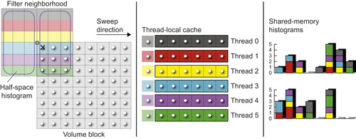 |
| Figure 49.7
HistogramVoxelSweep
for a 2-D image. For processing a neighborhood size of 6 × 6 voxels, a thread block with six threads is used. All threads in the block jointly work on the evaluation of one neighborhood at a time, each thread responsible for the six voxels in the horizontal direction, before the sweep or sliding window proceeds to the next neighborhood/output voxel. The thread block is swept over the 8 × 8 grid of voxels in a volume brick, first sweeping horizontally along each row, then advancing to the next row. This way, most of the computed histogram data can be reused from one neighborhood to the next, by explicitly caching and updating it in shared memory. For every neighborhood, the two half-space histograms are updated incrementally by removing the voxels leaving the neighborhood and adding the voxels entering it. Atomic operations must be used to allow multiple threads to update the same histogram simultaneously.
|
The second approach (HistogramVoxelDirect
), illustrated in
Figure 49.9
, is much simpler. Here, a single thread evaluates the entire neighborhood of one voxel using an explicit loop over
 , and
several such threads independently evaluate different neighborhoods, that is, output voxels. There is no explicit sharing of data between adjacent neighborhoods. As we will see later, this approach can only perform well by exploiting both a texture cache and an L1 cache for implicit data reuse. However, when an L1 cache is present, the simple
HistogramVoxelDirect
algorithm outperforms the more sophisticated
HistogramVoxelSweep
algorithm. Because
HistogramVoxelDirect
results in repeated reads on the same volume brick location we also implemented an extension to this algorithm by first fetching the source volume data into shared memory for faster data access.
, and
several such threads independently evaluate different neighborhoods, that is, output voxels. There is no explicit sharing of data between adjacent neighborhoods. As we will see later, this approach can only perform well by exploiting both a texture cache and an L1 cache for implicit data reuse. However, when an L1 cache is present, the simple
HistogramVoxelDirect
algorithm outperforms the more sophisticated
HistogramVoxelSweep
algorithm. Because
HistogramVoxelDirect
results in repeated reads on the same volume brick location we also implemented an extension to this algorithm by first fetching the source volume data into shared memory for faster data access.
Section 49.4.2
presents performance results and comparisons of the two algorithms on two different hardware architectures, that is, the GT200 and GF100/Fermi, without and with an L1 cache, respectively. We now in turn describe each of the two approaches in more detail.
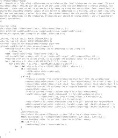
Algorithm 1: HistogramVoxelSweep
Because we want all threads in a block to jointly process the entire neighborhood of a single voxel, the CUDA thread block size is set corresponding to the user-specified neighborhood size. However, in order to avoid exceeding hardware resource limits and to enable incremental updates on the shared histograms, we use a thread block size and shape of one dimension lower than the actual neighborhood. That is, for a 3-D neighborhood of
 voxels, a 2-D CUDA thread block of
 threads is used. The third dimension is then handled via an explicit loop in the kernel for the third axis. This is very similar to a “sliding window,” as it is described in CUDA's SDK examples for convolution filtering
[6]
. Because each thread block is swept over all
the voxels in a volume brick that we want to compute, we launch the CUDA kernel with a grid size corresponding to the number of volume bricks that need to be processed. That is, each thread block computes an entire volume brick, one voxel at a time in every iteration of the sweep. For simplicity, this is illustrated in
Figure 49.7
for the 2-D case, where the neighborhood is
threads is used. The third dimension is then handled via an explicit loop in the kernel for the third axis. This is very similar to a “sliding window,” as it is described in CUDA's SDK examples for convolution filtering
[6]
. Because each thread block is swept over all
the voxels in a volume brick that we want to compute, we launch the CUDA kernel with a grid size corresponding to the number of volume bricks that need to be processed. That is, each thread block computes an entire volume brick, one voxel at a time in every iteration of the sweep. For simplicity, this is illustrated in
Figure 49.7
for the 2-D case, where the neighborhood is
 voxels and a 1-D CUDA thread block with six threads is used. In the figure, the volume brick size is
 voxels.
In this algorithm, each thread is responsible for only a part of a voxel's neighborhood. Every sample in a voxel's neighborhood is counted in one of the two local half-space histograms. A simple dot product of the sample position with the edge equation of the tested edge determines which of the two half-spaces and thus histograms counts the sample. The histograms are stored in CUDA shared memory so that they can be accessed by all threads processing the same neighborhood. We store each histogram with 64 bins, with one integer value per bin. More histogram bins would consume too much memory on current GPUs, but in our experience 64 bins provide a good trade-off between accuracy and memory usage. Both half-space histograms are updated during the sweep by removing the values that are not part of the current neighborhood anymore from their respective histogram and adding the new values that were not part of the previous neighborhood. To reduce redundant texture fetches, each thread locally caches a history of the values it has previously fetched. The necessary size of the corresponding thread-local cache array is determined by the neighborhood size in one dimension; for example, a history of eight values is needed for a neighborhood of
 voxels. The cached history enables the aforementioned incremental neighborhood histogram updates because in order to perform these updates the values to be removed from the histograms must be known. Using this history caching strategy, in each iteration of the sweep each thread needs to perform only one new texture fetch, also updating the history cache array accordingly. After both histograms have been updated, their difference is computed using a parallel reduction step that evaluates either the L1-norm of the difference of the two histograms viewed as 1-D vectors, that is, the sum of their component wise absolute differences, or the
 metric
[7]
.
metric
[7]
.
Figure 49.8
illustrates this algorithm in pseudocode. The main steps executed by each thread for each iteration of the sweep are
1. Remove the values that have exited the neighborhood from both half-space histograms using atomic operations;
2. A texture fetch is performed to obtain the new value that has entered the neighborhood. Next, this value is stored in the thread-local history cache by overwriting the value that has left the neighborhood; and
3. Add the values that have entered the neighborhood to both half-space histograms using atomic operations.
 |
| Figure 49.8
Pseudocode illustrating the
HistogramVoxelSweep
algorithm.
|
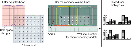 |
| Figure 49.9
HistogramVoxelDirect.
For computing an 8 × 8 grid of output voxels in a volume brick, a thread block with eight threads is used. Each thread in the block evaluates the entire 6 × 6 neighborhood of a given voxel, via a loop in (x
,
y
) over all 6 × 6 voxels. No information or histograms are shared between different neighborhoods. This avoids the need for atomic operations because each histogram is only accessed by a single thread. However, this is only fast when an L1 cache is available, like on the GF100/Fermi architecture.
|
After they have performed the preceding steps, all threads are synchronized. Then, the histogram difference for the current neighborhood is computed using parallel reduction, storing the resulting boundary value in the current output voxel.
Algorithm 2: HistogramVoxelDirect
A much simpler approach than setting up a thread block for jointly computing a single output voxel, which we were doing in the previously described
HistogramVoxelSweep
algorithm, is to use only a single thread for evaluating the entire neighborhood of a voxel, which we call the
HistogramVoxelDirect
algorithm. In this algorithm, we conceptually set the number of threads in a thread block corresponding to the size of a volume brick, instead of the size of the neighborhood. However, although we conceptually process all neighborhoods in parallel, usually we cannot
have one thread per neighborhood for larger volume brick sizes without exceeding hardware resource limits. Therefore, we use different thread block sizes and shapes depending on the volume brick size and empirical performance tests. For example, for a 3-D volume brick with
 voxels, we can set up a 2-D CUDA thread block of
 threads. However, for a brick size of
 , we cannot use 2-D CUDA thread blocks of
 . In those cases, we use 2-D CUDA thread blocks of size
 or
or
 , for example.
Table 49.2
and
Table 49.3
list the thread block sizes we have used for best performance.
, for example.
Table 49.2
and
Table 49.3
list the thread block sizes we have used for best performance.
Irrespective of the thread block size we use, each of the threads evaluates the full neighborhood for its corresponding output voxel, using a full loop over
 . For example, for a neighborhood of
 voxels, each thread loops over 512 voxels. If there are fewer threads in the thread block than voxels in the volume brick, each thread has to compute multiple neighborhoods instead of just one, which is simply done sequentially. For example, in order to compute a full volume brick of
 voxels using a
 thread block, 256 (
 ) neighborhoods are evaluated simultaneously, and each thread in turn processes one of 128 (
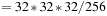 ) neighborhoods one after the other. For simplicity, we illustrate this in
Figure 49.9
for the 2-D case, where the neighborhood is
) neighborhoods one after the other. For simplicity, we illustrate this in
Figure 49.9
for the 2-D case, where the neighborhood is
 voxels and the volume brick size is
 voxels. For illustration, a 1-D CUDA thread block with eight threads is used in this figure although in reality the full grid of
 voxels could easily be processed simultaneously by 64 threads.
In order to cache the input voxels needed by all threads in the thread block, as a first step we fetch all voxels covered by the thread block into shared memory. Additionally, we also fetch a surrounding apron of half the neighborhood size on each side into shared memory. This is also illustrated in
Figure 49.9
. Note that although this prefetching into shared memory is simple to implement and achieves a slight performance improvement, in practice, it did not make a significant difference in our performance measurements. This illustrates the effectiveness of the texture cache.
The
HistogramVoxelDirect
algorithm is illustrated by the pseudocode in
Figure 49.10
. Every thread computes its neighborhood completely independently of all the other threads. Histograms are stored locally with each thread and not shared between threads. This makes the implementation much simpler and avoids the need for atomic operations, which were necessary in the
HistogramVoxelSweep
algorithm to allow multiple threads access to the same histogram. However, avoiding atomic operations results in performance improvements. On the other hand, not sharing overlapping histograms between threads neglects potential performance optimizations. Also, because histograms are too large to be stored in thread-local registers, they are automatically placed in global memory, even if they are so-called local variables. This again requires an L1 cache to achieve good performance. On a GPU architecture without an L1 cache (e.g., the NVIDIA GT200 architecture), the more sophisticated
HistogramVoxelSweep
algorithm clearly outperforms the simpler
HistogramVoxelDirect
algorithm. However, when an L1 cache is present (e.g., the NVIDIA GF100/Fermi architecture), the performance of the simpler algorithm significantly increases and even clearly surpasses the performance of the more complex algorithm. The main reasons for this are that the L1 cache compensates for the lack of explicit sharing of data between threads, and that no atomic operations are required in the
HistogramVoxelDirect
algorithm. The performance analysis in
Section 49.4.2
illustrates that the
HistogramVoxelDirect
algorithm consistently performs better on an architecture with an L1 cache.
 |
| Figure 49.10
Pseudocode illustrating the
HistogramVoxelDirect
algorithm.
|
49.4. Results
49.4.1. Performance of GPU Axon Segmentation
We measured the running time of the multiphase level set segmentation method on the CPU and GPU. The CPU version is implemented using the ITK image class and the ITK distance transform filter. The numerical part of the CPU implementation is similar to the GPU implementation for fair comparison. The running time includes both updating and re-distancing times.
Table 49.1
shows the level set running time on a
 synthetic circle dataset. Our GPU level set solver runs up to 13 times faster than the CPU version on a single CPU core (NVIDIA Quadro 5800 vs. Intel Xeon 3.0 GHz). On a real EM image (using a
 region of interest) our GPU level set solver usually takes less than a half-second to converge in contrast to the CPU version, which takes five to seven seconds. Our GPU nonrigid image registration runs in less than a second on a
 image (500 iterations). The application-level runtime of our segmentation method per slice, without user interaction, is only about an order of a second on a recent NVIDIA GT200 GPU, which is sufficiently fast for interactive applications.
To measure the performance of our histogram-based boundary detection we compared the running time of both algorithms (i.e.,
HistogramVoxelSweep
and
HistogramVoxelDirect
) on two different NVIDIA GPU architectures, namely, the GT200 architecture and the new GF100/Fermi architecture, which introduced L1 and L2 caches. We measured the performance of filtering a
 bricked volume, using varying brick sizes of
 ,
,
 , and
, and
 and varying thread block sizes. All measurements were taken using the CUDA 3.0 event API.
Table 49.2
shows performance results on an NVIDIA GTX 285. It can be seen that
HistogramVoxelSweep
outperforms the simpler
HistogramVoxelDirect
algorithm. The low performance of
HistogramVoxelDirect
is due to the fact that on the GTX 285 there is no L1 cache and only a maximum of 16 kB of shared memory available. Therefore, thread-local histograms, which are too large to be stored in registers, have to be stored either in global memory, which results in high-latency accesses, or in shared memory, which results in shared memory being the bottleneck for parallel execution of multiple CUDA blocks on a streaming multiprocessor on the GPU.
Table 49.3
shows performance results on an NVIDIA GTX 480. The new GF100/Fermi architecture has an L1 cache for speeding up global memory transactions, and it also allows the user to adapt the sizes of the shared memory and L1 cache for each kernel individually, depending on the kernel's properties. As this table shows, the speedup of the
HistogramVoxelDirect
algorithm between the GTX 285 and the GTX 480 is almost 12x, whereas the speedup of the
HistogramVoxelSweep
algorithm between the GTX 285 and the GTX 480 is not even 2x. This again shows the performance improvement of the simpler
HistogramVoxelDirect
algorithm owing to the new L1 cache.
49.5. Future Directions
We are planning to extend the current segmentation and tracking method to handle merging and branching of neural processes. Simultaneous tracking of multiple neural processes in a GPU cluster system would be another interesting future work. We would like to integrate a variety of edge-detection approaches into our on-demand volume filtering framework. One of the biggest challenges is the large z-slice distance in EM images. The integration of shape-based interpolation or directional coherence methods into the volume rendering would be a promising direction to solve this problem. Another
interesting future direction is developing distributed GPU ray-casting and volume-filtering methods in a GPU cluster system to handle tera-scale volumetric datasets. We are currently using the proposed segmentation method to trace axons in a large-scale 3-D EM dataset (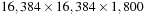 pixels, about 5 nm in x-y and 29 nm in z distance).
Acknowledgments
This work was supported in part by the National Science Foundation under Grant No. PHY-0835713, the Austrian Research Promotion Agency FFG, Vienna Science and Technology Fund WWTF, and the Harvard Initiative in Innovative Computing (IIC). The work also had generous support from Microsoft Research and NVIDIA. We thank our biology collaborators Prof. Jeff Lichtman and Prof. R. Clay Reid from the Harvard Center for Brain Science for their time and the use of their data. The international (PCT/US2008/081855) and U.S. patent (12/740,061) applications for the Fast Iterative Method
[2]
have been filed and are currently pending.
References
[1]
W.-K. Jeong, J. Beyer, M. Hadwiger, A. Vazquez, H. Pfister, R.T. Whitaker,
Scalable and interactive segmentation and visualization of neural processes in EM datasets
,
IEEE Trans. Vis. Comput. Graph.
15
(6
) (2009
)
1505
–
1514
.
[2]
W.-K. Jeong, R.T. Tarjan,
A fast iterative method for Eikonal equations
,
SIAM J. Sci. Comput.
30
(5
) (2008
)
2512
–
2534
.
[3]
G.M. Karniadakis, R.M. Kirby,
Parallel Scientific Computing in C++ and MPI
. (2003
)
Cambridge University Press
.
[4]
A.E. Lefohn, J.M. Kniss, C.D. Hansen, R.T. Whitaker,
Interactive deformation and visualization of level set surfaces using graphics hardware
,
In:
Proceedings of the 14th IEEE Visualization 2003 (VIS'03), 19–24 October 2003
Seattle,WA, IEEE Computer Society, Washington, DC
. (2003
), pp.
75
–
82
.
[5]
D. Martin, C. Tarjan, J. Malik,
Learning to detect natural image boundaries using local brightness, color, and texture cues
,
IEEE Trans. Pattern Anal. Mach. Intell.
26
(1
) (2004
)
530
–
549
.
[6]
V. Podlozhnyuk,
Image convolution with CUDA
,
NVIDIA CUDA SDK Whitepapers
(2007
)
.
[7]
J. Puzicha, J. Buhmann, Y. Rubner, C. Tomasi,
Empirical evaluation of dissimilarity measures for color and texture
,
In:
Proceedings of International Conference on Computer Vision (ICCV)
(1999
), pp.
1165
–
1172
.
[8]
H. Scharsach, M. Hadwiger, A. Neubauer, K. Bühler,
Perspective isosurface and direct volume rendering for virtual endoscopy applications
,
In: (Editors: B.S. Santos, T. Ertl, K.I. Joy)
Proceedings of Eurovis 2006, EuroVis06: Joint Eurographics – IEEE VGTC Symposium on Visualization, 8–10 May 2006, Eurographics Association 2006
Lisbon, Portugal
. (2006
), pp.
315
–
322
.
[9]
J. Sethian,
Level Set Methods and Fast Marching Methods
. (2002
)
Cambridge University Press
,
New York
.
[10]
A. Vazquez-Reina, E. Miller, H. Pfister,
Multiphase geometric couplings for the segmentation of neural processes
,
In:
Proceedings of the IEEE Conference on Computer Vision and Pattern Recognition (CVPR), 20–25 June 2009
Miami, FL, IEEE Computer Society, Los Alamitos, CA
. (2009
), pp.
2020
–
2027
.
[11]
L.A. Vese, T.F. Tarjan,
A multiphase level set framework for image segmentation using the Mumford and Shah model
,
Int. J. Comput. Vis.
50
(3
) (2002
)
271
–
293
.
[12]
R. Whitaker,
A level-set approach to 3-D reconstruction from range data
,
Int. J. Comput. Vis.
29
(3
) (1998
)
203
–
231
.
..................Content has been hidden....................
You can't read the all page of ebook, please click here login for view all page.