
Aircraft Weight Analysis
Abstract
A number of methods to estimate various weights associated with aircraft are presented. Definitions of important weight properties, such as empty, gross, ramp, and maximum zero fuel weight are defined. Two weight estimation methods, intended to assess the first estimate of the airplane’s weight based on historical data, are introduced using numerical examples. Then, three detailed weight analysis methods referred to as actual, statistical, and direct weight estimation methods are presented. Statistical methods associated with Raymer and Nicolai are introduced. Also a methodology called Method of Fractions is introduced to relate wing weight to its AR, but such methods are helpful in establishing relationships for optimization approaches. The last section of the chapter presents many important inertia properties, including numerical estimation of moments and products of inertia, prediction of the aircraft’s 3D CG location, and others. Additionally, the CG-envelope and its creation are detailed; along with a discussion of in-flight movement, weight budgeting and tolerancing methods.
Keywords
Empty; design gross; crew; fuel; ramp; maximum landing; maximum zero fuel weight; payload; useful load; weight ratio; initial weight estimation; detailed weight analysis; statistical; CG envelope; center of gravity; center of mass; moment of inertia; product of inertia; loading cloud; weight budget; weight tolerances
Outline
A Comment About Units of Weight
6.1.1 The Content of this Chapter
Useful Load − Wu = Wuseful load
Maximum Zero Fuel Weight − WMZF
6.1.3 Fundamental Weight Relations
6.2 Initial Weight Analysis Methods
6.2.1 Method 1: Initial Gross Weight Estimation Using Historical Relations
6.2.2 Method 2: Historical Empty Weight Fractions
6.3 Detailed Weight Analysis Methods
6.4 Statistical Weight Estimation Methods
6.4.1 Method 3: Statistical Aircraft Component Methods
Air-conditioning and Anti-icing
6.4.2 Statistical Methods to Estimate Engine Weight
6.5 Direct Weight Estimation Methods
6.5.1 Direct Weight Estimation for a Wing
6.5.2 Variation of Weight with AR
Baseline Definitions for a Trapezoidal Wing
6.6.4 Moment About (X0, Y0, Z0)
6.6.5 Center of Mass, Center of Gravity
6.6.6 Determination of CG Location by Aircraft Weighing
6.6.7 Mass Moments and Products of Inertia
Parallel-axis Theorem for Moments of Inertia
Parallel-plane Theorem for Products of Inertia
6.6.8 Moment of Inertia of a System of Discrete Point Loads
6.6.9 Product of Inertia of a System of Discrete Point Loads
6.6.11 Center of Gravity Envelope
6.6.12 Creating the CG Envelope
Determination of the Aft CG Limit
Determination of the Forward CG Limit
6.1 Introduction
One of the most important steps in the aircraft design process is the estimation of the weight of the vehicle. While usually not requiring complicated mathematical tools, this task can bring considerable challenges for the cognizant engineer. One of the challenges is that excessive under- or overestimation of an airplane’s empty weight can bring dire consequences to a development program. Weight-related issues in aircraft development programs have been brought to the forefront recently by the Lockheed-Martin F-35, which allegedly was nearly 3000 lbf over target. On April 7, 2004, Lockheed declared a stand-down day, notifying its employees that further development of the aircraft would halt until the weight was lost [1]. A number of problems were introduced – if its gross weight was allowed to stand, it would suffer a reduction in useful load. If it was increased, the reduced thrust-to-weight ratio would lead to detriments in performance and render it unable to accomplish its advertised short take-off vertical landing (STOVL) capability.
The history of aviation is wrought with overweight aircraft. In civilian circles the two latest are reports of the Boeing 787 Dreamliner [2] and Airbus 380 [3]. If these established manufacturers can make mistakes in their estimations, then certainly we can too. This section introduces several methods to help the designer estimate the weight of the airplane. The complexity and accuracy of these methods vary. The simplest ones are intended for initial estimation only and their accuracy will only land you in the ballpark. As one would expect, the more complex methods are more accurate, but also depend on some specific knowledge about the geometry and other parameters, such as wing area, quantity of fuel, or length of landing gear. Therefore, they can only be used once the primary dimensions of the aircraft have been established.
As detailed in Section 1.3, Aircraft design algorithm, a new estimate of the weight is required during each design iteration. The first iteration calls for a simple weight estimate to be performed and this can be accomplished using either of the two methods presented here. Both are based on historical data and assume the class of the aircraft is known. These methods will only give a rudimentary idea as to how heavy the airplane may become and are intended to allow basic sizing to take place. The second set of methods are more detailed estimations that usually include a mixture of known weights (such as for engines, landing gear components, etc.), statistical weights, and direct weight estimation (based on the geometry and density of materials chosen).
Once the design iterations begin, the designer should update all calculations that refer to the previous weight, as stipulated in Section 1.3.
Initial Weight Estimation
Initial weight analysis methods are only intended to be used during the first iteration of the airplane design. The estimation of the weight is equally important to that of the drag. Overly optimistic weight estimation has killed a number of design programs in the history of aviation and is an engineering problem that is not likely to become a “thing of the past” for the foreseeable future. This section will present some helpful methods to get you started with your new design; however, you must advance into more sophisticated methods during subsequent design iterations.
Detailed Weight Estimation
Detailed weight analysis is performed during the second and any subsequent iteration. It is one of the most important tasks in the design process and must be approached with great care and seriousness. A flawed analysis can contribute to a program cancellation. The most common pitfall is underestimating the empty weight, as stated under maximum zero fuel weight – WMZF below. This section discusses methods used to correctly estimate a likely empty weight of an aircraft, but the reader should be aware that their proper use demands great engineering judgment.
Weight Estimation Advice
Be realistic: do not expect your design to weigh less than airplanes in a similar class – at least not for the first iteration. The aircraft that you’re comparing with have often gone through costly weight-reduction programs and many can be considered largely weight-optimized. Remember that the people who worked on these aircraft were smart people as well and probably spent a lot of time trying to get unnecessary weight out. Your design will not be optimized at first.
Be careful: if your airplane ends up weighing less than planned, then great – it will have greater utility or growth capacity than planned and your boss may even pat you on the back. If your airplane ends up heavier than planned, don’t be surprised if the project is cancelled. That’s really how simple it is, although you would most likely be asked to sharpen your pencil first.
A Comment About Units of Weight
Weight is a force. Its unit in the UK system is lbf, pronounced “pounds” or “pounds-force”. In the SI system, the correct unit is N, pronounced “newtons.” Most metric countries, while technically incorrect, specify weight using the unit of mass – kg (kilograms), rather than newtons. This way, an airplane is specified to “weigh,” say 906 kilograms (or kilos) and not 19,614 N (which corresponds to 2000 lbf). For this reason, when referring to the weight of aircraft using the metric system, this convention will be adhered to. The reader is reminded to keep this convention in mind when coming across weight stated as a unit of mass.
6.1.1 The Content of this Chapter
• Section 6.2 presents two methods intended to assess the first estimate of the airplane’s weight.
• Section 6.3 discusses detailed weight analysis methods, a precursor to the statistical and direct weight estimation methods.
• Section 6.4 presents a method to estimate the weight of GA aircraft.
• Section 6.5 presents direct weight estimation methods.
• Section 6.6 discusses the various inertia properties, including numerical estimation of moments and products of inertia. The importance of weight budgeting in aircraft design is presented, as well as methods to evaluate uncertainty in the prediction of the CG and other inertia properties.
6.1.2 Definitions
The following are standard definitions for weight used in the aircraft industry.
Empty Weight − We = Wempty
Weight of an aircraft without useful load. Includes oil, unusable fuel, and hydraulic fluids.
Design Gross Weight − W0
The maximum T-O weight for the mission the airplane is designed for.
Useful Load − Wu = Wuseful load
Useful load is defined as the difference between the design gross weight and the empty weight. It is the weight of everything the aircraft will carry besides its own weight. This typically includes occupants, fuel, freight, etc.
Payload − Wp = Wpayload
The part of the useful load that yields revenue for the operator. Typically it is the passengers and freight.
Crew Weight − Wc = Wcrew
Weight of occupants required to operate the aircraft.
Fuel Weight − Wf = Wfuel
Weight of the fuel needed to complete the design mission.
Ramp Weight − WR = Wramp
Design gross weight + small amount of fuel to accommodate warm-up and taxi into T-O position.
Maximum Landing Weight − WLDG
Maximum weight at which the aircraft may land without compromising airframe strength.
Maximum Zero Fuel Weight − WMZF
Max zero fuel weight is the maximum weight the airplane can carry with no fuel on board. Note that the maximum zero fuel weight implies that all weight above WMZF lbs must be fuel.
Of the above definitions, only last of these requires elaboration. It is a relatively common occurrence in the aviation industry that gross weight must be increased. There are typically two underlying reasons for this: (1) the design team underestimated the gross weight, and (2) it is desired that the airplane is capable of being operated at a greater weight than initially anticipated. Note that from a certain point of view, the second reason is a different version of the first reason.
So, consider the predicament confronting a hypothetical design team after initially estimating the empty and gross weight of a new airplane to be 3000 lbf and 5000 lbf, respectively. This means a useful load of 2000 lbf. Then one day, during the detail design phase, as the design team is meticulously trying to comply with aviation regulations and accommodate management and customer requests for added features, the weights engineer drops a bomb during a design review meeting announcing that there is no way the gross weight target can be met! This airplane will weigh 3500 lbf empty! Based on the numbers above it is easy to see that this sudden and unwelcome injection of reality means the projected useful load just dropped from 2000 to 1500 lbf – a whopping one-quarter, eradicating the design’s competitive edge! So, what can be done? Should the wing area be increased? Since the wings may already have been designed, this implies a major redesign effort with associated delay in delivery and costs. Perhaps the weights engineer should be fired? Well, a new one will have to be hired and he or she will probably only repeat the bad news, so this won’t help. Should a major structural optimization be initiated in the hope that 500 lbf of lard can be found and designed out of the airplane? If the airframe design is being accomplished by an experienced engineering team it is unlikely there will be more than 50–100 lbf of extra weight at this stage – and it will be costly and also delay delivery. It is then that a knowledgeable engineer in the group saves the day by suggesting the concept of WMZF. This change is mostly a matter of paperwork and is contingent on the approval of the aviation authorities. If approved, it works as follows and as illustrated in Figure 6-1:
(1) In order to maintain the same competitive useful load of 2000 lbf, the best choice is to increase the gross weight from 5000 to 5500 lbf.
(2) If the fuel is carried in the wings it will act as a bending moment relief and, therefore, not require a change in its internal structure.
(3) A large number of loading combinations are studied during the design in the form of so-called load cases (or load conditions). As an example, one of the load cases would consist of the airplane with fuel tanks filled to the brim and a few passengers on board; in another load case, all of that fuel has been consumed; and in a third, the airplane is filled with passengers and has very little fuel, and so forth. And it would be shown for all the load combinations that the airframe does indeed comply with aviation regulations. For this reason, it can be argued that this airplane may be loaded indiscriminately up to 5000 lbf; however, once there, all remaining weight (500 lbf) must be fuel in the wing. If this is done, then it can be argued that the weight of the fuel will counter the added aerodynamic load that the wing must generate and react. To see this, assume we add 250 lbf of fuel to each wing. This weight calls for a 250 lbf increase in lift, canceling the impact on the shear force that must be reacted. In other words, once airborne, the stress in the spar caps, skin, and shear webs is effectively unchanged.

This elementary physics is often surprisingly hard for many to grasp. So consider the following thought experiment. Imagine an extremely light wing model inside a wind tunnel and at a given airspeed and AOA, some 100 lbf of lift is measured. This means that the wing attachment is reacting 100 lbf in shear, right? Now, consider a new model of this wing is installed in the tunnel, except this one weighs 100 lbf. When run at the same airspeed and AOA as the previous model, what is the shear force reacted by the wing attachment? 100 lbf? 0 lbf? If you said 0 lbf, you are correct. By the same token, if 25 lbf of weight is now added to the wing (so it weighs 125 lbf) and it is made to generate 125 lbf of lift, the same thing happens; again the net shear being reacted by the attachment is 0 lbf. From the standpoint of the material in the attachment, it sees exactly the same magnitude of stresses in either case.
Of course it's not so simple in practice. There are other consequences of the maximum zero fuel weight. One is an increase in the stalling speed, which, as a consequence of this approach, may call for a redesign of the high-lift system (which is easier than redesigning the entire wing). The other is reputation. The very concept implies some mistakes in weight estimation may have been made along the way, whether this is true or not. Regardless, the concept of maximum zero fuel weight is something the aircraft designer should be aware of and understand. This can come in very handy when least expected.
6.1.3 Fundamental Weight Relations
The following relations are fundamental expressions for an aircraft weight. In comparing Equations (6-1) and (6-3), the reader should be mindful that Equation (6-1) is a primary governing equation and (6-3) is an expression of what the useful load might consist of.
Note that Equation (6-1) gives the maximum or “official” Wu, while Equation (6-2) gives the “current” Wu. It may or may not be equal to the “official” Wu. Weight ratios are imperative in estimating the weight during the first design iteration, but are also necessary for mission analyses. The fundamental weight ratios are the empty weight and fuel weight ratios:
6.1.4 Mission Analysis
When designing aircraft to specific missions, where range or endurance requirements are clearly spelled out, it becomes imperative to assess the amount of fuel required to complete the mission. Mission analysis is a tool intended to help assess the amount of fuel for this purpose. This tool is imperative during the conceptual design stage and is closely related to the estimation of range and endurance. For this reason, further discussion is presented in Section 20.5, Analysis of mission profile.
6.2 Initial Weight Analysis Methods
Before beginning serious development on a new aircraft it is absolutely imperative to review the weight of aircraft that belong to the same class as the proposed design. Since such work focuses on historical aircraft, the formulations that result are referred to as historical relations. These are typically ratios, for instance, empty and fuel weight ratios. They are based on the assumption that the new airplane will be certified using similar regulations as the historical reference aircraft and, therefore, must react identical load factors. Consequently, as long as the new aircraft carries a similar payload, is similarly configured, and made from similar materials as the reference aircraft, their weights are likely to be similar. The accuracy of these methods depends on the number of reference aircraft and how closely they resemble the one being drafted.
6.2.1 Method 1: Initial Gross Weight Estimation Using Historical Relations
Guidance: Use this method if the gross weight is not known beforehand. Be careful – it can yield an over-estimation. Ensure that the reference aircraft database consists of aircraft in the same class and is not a mix of properties. For instance, if designing a piston-propeller aircraft, do not mix turboprop or turbofan aircraft in the database. Also, do not mix small two-place and large 19-place aircraft, or low-performance VFR and high-performance IFR aircraft, and so on.
Consider the design of a new 6-seat, twin-engine, piston-powered aircraft. It fits perfectly into the class of twin-engine GA aircraft – or does it? This class includes other twin-engine aircraft such as the Piper PA-23 Apache, Beech Model 76 Duchess, Beech Model 58 Baron, Piper PA-31 Navajo, Cessna Model 303, and Cessna Model 421. The empty weight of these aircraft ranges from about 3200 to 4500 lbf and the gross weight from 5200 to 7500 lbf. They are all powered by a number of different piston engine types, and carry different amounts of payload, from six to eight occupants or so. It is prudent to include these aircraft in the statistical analysis. However, the Piper PA-42 Cheyenne or the Beech Model 100 King Air, not to mention its larger relatives, the Model 200 and 300 Super King Air, should be excluded. These aircraft weigh some 6900 to 7800 lbf empty; 11,200 to 12,500 lbf loaded; and are powered by gas turbines, are pressurized, and of higher performance than the aforementioned aircraft. The point being made is that the selection of candidate aircraft must be refined enough to exclude aircraft that either have or lack features that could skew the results. In the case of the above aircraft we have major differences in properties such as pressurized versus unpressurized, piston engine versus turbine, and so forth.
Besides serving as a “sanity check” and, thus, possibly preventing disastrous consequences of under- or overestimating the weight, selective inclusion and exclusion of candidate aircraft improves the reliability and allows a realistic “first stab” estimation of the airplane’s gross weight to take place. First, however, the fuel and empty weight ratios must be defined.
Once these have been established, we can rewrite the expression for the design gross weight as the sum of the empty weight, crew weight, fuel weight, and payload:
![]() (6-8)
(6-8)
This can be solved for W0, yielding an expression that can be used to estimate gross weight in terms of the weight ratios.
![]() (6-9)
(6-9)
Then, the gross weight is estimated as follows: (1) Establish the desired payload, Wp, and crew weight, Wc, for the new design. (2) Determine historical values for fuel and empty weight ratios of similar aircraft. (3) Calculate the proposed gross weight using Equation (6-9).
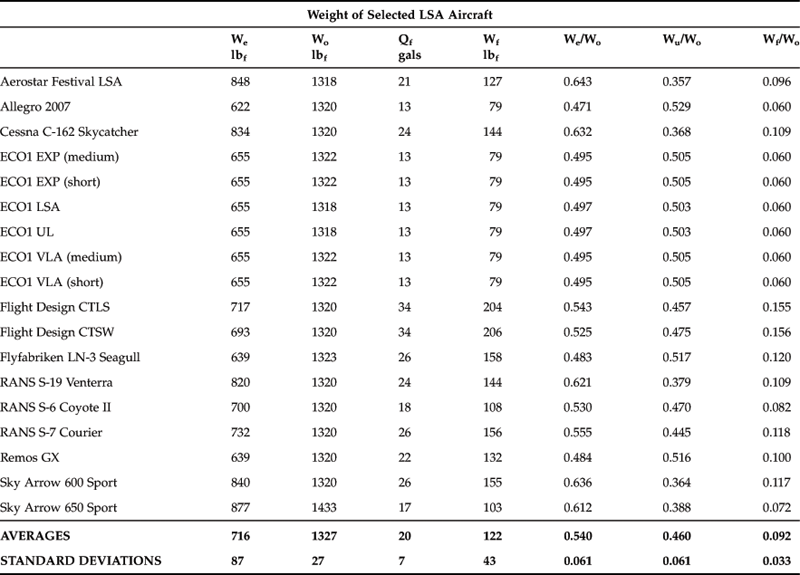
The ratios We/W0 and Wf/W0 can be obtained from historical data, providing a possible solution to Equation (6-9). Relationships for We/W0 are provided by Raymer [4], Torenbeek [5], and Nicolai [6]. The ratio Wf/W0 is best obtained by research into similar aircraft. Additionally, aircraft specifications in the public domain, such as those found in Jane’s All the World’s Aircraft or on type certificate data sheets, can be used to build such relationships. Table 6-1 shows an example of such analysis for a number of light sport aircraft. Note that We stands for empty weight, Wu is useful load, Wf is fuel load, and W0 is gross weight.
TABLE 6-1
Establishing Weight Ratios for Light Sport Aircraft
Sources of data are various manufacturers' websites. Data may contain erroneous weights.
The statistical values in Table 6-1 suggest that the empty weights of the selected aircraft are 716 ± 87 lbf and the gross weights 1327 ± 27 lbf. Furthermore, for the designer of an LSA aircraft, it suggests an empty weight ratio, useful load ratio, and fuel weight ratio of around 0.540, 0.460, and 0.092, respectively. This information is vital for the initial sizing, for instance when performing constraint analysis. Statistical equations for a number of classes of aircraft are presented below in Section 6.2.2, Method 2: Historical empty weight fractions.
NB: Many real airplanes exceed their gross weight with all seats loaded and full fuel tanks. This way, an airplane may be capable of a fuel weight ratio of 0.20, but only 0.10 if all seats are occupied. Using the former value with Equation (6-9) would therefore yield gross weight that is unrealistically high. For this reason, the reader is urged to exercise caution and select the value of Wf/W0 accordingly. For instance, adjust the historical fuel weight ratio by simply calculating Wf = W0 − We − Wp − Wc and compute an adjusted Wf/W0. Alternatively, the designer is at liberty to decide that when all seats are occupied, the airplane can hold some specific quantity of fuel that may or may not refer to full fuel tanks. This, by the way, is not done in Example 6-2 below, and explains why the gross weight is so unrealistically high.
EXAMPLE 6-2
A four-seat trainer is being designed and it is required to carry 300 lbf of baggage in addition to the occupants. Assume a crew of one, 200 lbf/person, and use the ratios We/W0 and Wf/W0 obtained from the analysis of the Cessna 150 in Example 6-1. For the conceptual design estimate initial values for:
6.2.2 Method 2: Historical Empty Weight Fractions
Guidance: Use this method if the gross weight is known beforehand. This is the case for many types of aircraft, e.g. LSA, which should not weigh more than 1320 lbf or 1430 lbf if amphibious. Do not “back out” W0 from a desired empty weight ratio using this method.
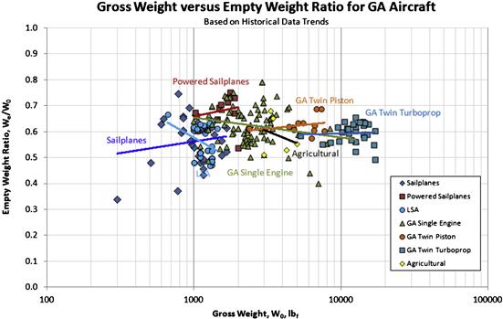
The modern aerospace engineer is in the enviable position of having access to a large collection of different kinds of airplanes to compare the design to (Figure 6-2). This is priceless during the conceptual design phase, when one or more airplanes can typically be found that compare well to the one being designed. In particular, this is helpful when it comes to estimating weight. Empty weight fractions are an important early step in the design process and people have devised statistical formulas based on historical aircraft that allow an initial empty or gross weight to be estimated by a class of aircraft.
Sailplanes:
![]() (6-10)
(6-10)
Powered sailplanes:
![]() (6-11)
(6-11)
Light sport aircraft (land):
![]() (6-12)
(6-12)
Light sport aircraft (amphib):
![]() (6-13)
(6-13)
GA single-engine:
![]() (6-14)
(6-14)
GA twinpiston:
![]() (6-15)
(6-15)
GA twin turboprop:
![]() (6-16)
(6-16)
Agricultural:
![]() (6-17)
(6-17)
6.3 Detailed Weight Analysis Methods
Upon completion of the first design iteration1, which yields the initial weight estimate, it is now time for the design team to sharpen their pencils and begin the estimation of a more accurate empty weight for the aircraft. The initial weight estimate should only be considered a value that gives an “idea of the weight” until the detailed weight analysis is completed.
During the second (and even subsequent) design iterations, things change frequently and this can pose problems for any trade study. An effective weight analyst will therefore try to create relationships between size and weight of airplane parts, as this will be of great help to those conducting trade studies. As an example, such relationships should allow the user to estimate the weight of the proposed design as a function of parameters such as wing area or number of occupants, and so on.
Another important result of weight analysis is information that allows weight budgeting to be prepared. The process will yield weight for components such as the wing, HT, VT, fuselage, etc., which can then be used to establish target weights for the components. It is of utmost importance that the structural design team is aware of the weight target of the structure as this will help in directing the design toward a lighter one. Weight targeting via weight budgeting is discussed in some detail in Section 6.6.14, Weight budgeting.
Typically, detailed weight estimation methods include:
| Known weights | –this section |
| Statistical weight estimation | –see Section 6.4 |
| Direct weight estimation | –see Section 6.5 |
The concept “known weights” refers to parts and components that can either be weighed with reasonable accuracy or whose manufacturer (if the component is obtained from an outside vendor) can disclose with reasonable confidence. Most of the time the weight analyst uses all three methods simultaneously, but known weights always supersede both the statistical and direct weight estimations. The following parts can be expected to have published weights:
Statistical and direct weight estimations will now be treated in some detail.
6.4 Statistical Weight Estimation Methods
Statistical weight estimation methods are based on historical data derived from existing airplanes. For instance, if we know the weight of the wing structure for a population of aircraft that fall into a specific class (e.g. twin-engine propeller aircraft), it is possible to derive relationships that could be based on geometric parameters such as wing area, aspect ratio, and taper ratio, as well as limit or ultimate load factors. The assumption is that the wing weight of two types of aircraft in the same class that are certified to the same set of regulations and whose gross weight is similar should be similar, even if made by different manufacturers. The statistical relationship established by the entire class of aircraft can thus be used to estimate the wing weight of any aircraft of the same class as long as it falls between the extremes of the aircraft in that class. Such estimation methods usually require some dimensions to have been established beforehand (e.g. AR, TR, sweep, S, etc.). Such methods are often developed in industry or in academia. Since many airplanes feature aluminum and composites alike, the user must use such statistical methods with care, as these may be solely based on aluminum aircraft.
Statistical weight estimation methods are always based on a specific class of aircraft, for instance, GA aircraft, commercial aircraft, fighters, and so on. Such classes share commonalities that improve the accuracy of the formulation. However, be mindful that some classes of aircraft have seen advances, such as an increased use of composites, that may skew the resulting weights.
6.4.1 Method 3: Statistical Aircraft Component Methods
Guidance: Only use this method once you have more information about the geometry of the aircraft. This is not an initial weight estimation method like methods 1 and 2, presented earlier; it requires a large amount of data that results from analysis that follows the use of those methods. It is to be used after! Also note that this method yields the empty weight, We, of the aircraft. To get the gross weight, W0, occupants, freight, and fuel must be added.
The following equations are presented in Raymer [4] and Nicolai [6] and are intended for conventional GA aircraft only. Both references cite their primary sources for these methods and both provide estimation methods for other aircraft types besides GA aircraft. The interested reader is directed to those sources for further details.
Note that the equations must be used with care as they are unit-sensitive; e.g. some arguments are in ft, while others are in inches. Also, the reader may ask: “Which method should I select, and why?” The short answer is that both methods should be used and, when possible, engineering judgment should be used to narrow down the two options. In some cases, the average of the two values should be pondered. In other cases, the two methods present identical equations (because they come from the same original source). The reader is strongly urged to apply it to a number of aircraft in the same class and evaluate how “close” it matches their empty weight. If the results do not match well, the results should be used to develop scaling factors. For instance, if the predicted weight is, say, 25% lighter than the actual empty weight of the reference aircraft, the results for the new aircraft should be multiplied by a factor of 1.25.
Wing Weight
Raymer:
![]() (6-18)
(6-18)
Nicolai:
 (6-19)
where
WW = predicted weight of wing in lbf
SW = trapezoidal wing area in ft2
WFW = weight of fuel in wing in lbf (If WFW = 0 then let ![]() )
)
AR = Aspect Ratio of wing, HT, or VT, per the appropriate subscripts
q = dynamic pressure at cruise
t/c = wing thickness to chord ratio
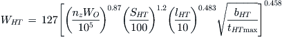
Horizontal Tail (HT) Weight
Raymer:
![]() (6-20)
(6-20)
Nicolai:
 (6-21)
where
Vertical Tail (VT) Weight
Raymer:
![]() (6-22)
(6-22)
Nicolai:
 (6-23)
where
Fuselage Weight
Raymer:
![]() (6-24)
(6-24)
Nicolai:
![]() (6-25)
(6-25)
where
WFUS = predicted weight of the fuselage in lbf
SFUS = fuselage wetted area in ft2
lFS = length of fuselage structure (forward bulkhead to aft frame) in ft
dFS = depth of fuselage structure in ft
VP = volume of pressurized cabin section in ft3
Main Landing Gear Weight
Raymer:
![]() (6-26)
(6-26)
Nicolai:
![]() (6-27)
(6-27)
where
Nose Landing Gear Weight
Raymer:
![]() (6-28)
(6-28)
where
WNLG = predicted weight of the nose landing gear in lbf
nl = ultimate landing load factor
Installed Engine Weight
Raymer:
![]() (6-29)
(6-29)
Nicolai:
![]() (6-30)
(6-30)
where
Fuel System Weight
Raymer:
![]() (6-31)
(6-31)
Nicolai:
![]() (6-32)
(6-32)
where
Flight Control-system Weight
Raymer:
![]() (6-33)
(6-33)
Nicolai:
![]() (6-34)
(6-34)
where
Hydraulic System Weight
Raymer:
![]() (6-35)
(6-35)
where
Avionics Systems Weight
Raymer:
![]() (6-36)
(6-36)
Nicolai:
![]() (6-37)
(6-37)
where
Electrical System
Raymer:
![]() (6-38)
(6-38)
Nicolai:
![]() (6-39)
(6-39)
Air-conditioning and Anti-icing
Raymer:
![]() (6-40)
(6-40)
Nicolai:
![]() (6-41)
(6-41)
where
Furnishings
Raymer:
![]() (6-42)
(6-42)
Nicolai:
![]() (6-43)
(6-43)
where
WFURN = predicted weight of furnishings in lbf
qH = dynamic pressure at max level airspeed, lbf/ft2
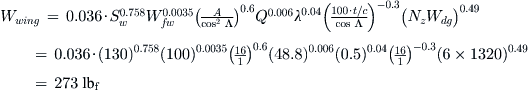
EXAMPLE 6-3
Determine the wing weight for a light airplane with the following specifications:
NZ = ultimate load factor = 1.5 × 4.0 = 6.0g
Q = dynamic pressure at cruise = 0.5 × 0.002378 × (120 × 1.688)2 = 48.8 lbf/ft2
SW = trapezoidal wing area = 130 ft2
t/c = wing thickness to chord ratio = 0.16
Wdg = design gross weight = 1320 lbf
Solution
Wing weight:
6.4.2 Statistical Methods to Estimate Engine Weight
The following methods have been derived based on a large number of piston, turboprops, and turbofans. These weights correspond to WENG in Equations (6-29) and (6-30). They are based on manufacturers' data.
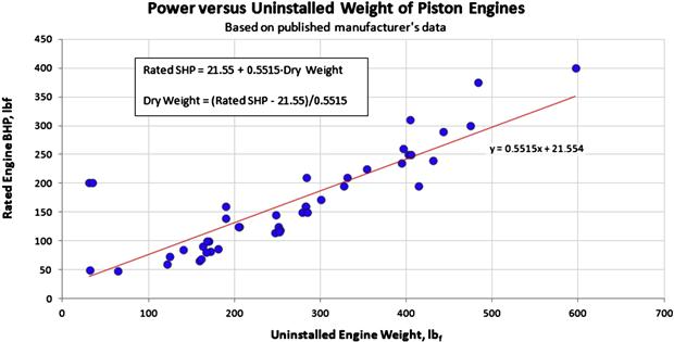
Weight of Piston Engines
Figure 6-3 shows the correlation between the uninstalled weight and rated brake horsepower of a variety of current piston engines. It is helpful for the designer when estimating the weight of a new engine, for instance, during the weight estimation phase or for multi-disciplinary optimization. Numerical analysis of the data reveals that if some specific rated BHP is being sought, the weight of the resulting engine can be estimated from:
Weight of Turboprop Engines
Figure 6-4 shows the correlation between the uninstalled weight and rated shaft-horsepower of a variety of current turboprop engines. This is a helpful tool for the designer, when a new engine is being developed for a specific application whose weight remains to be established. Numerical analysis of the data reveals that if some specific rated SHP is being sought, the weight of the resulting engine can be estimated from:
where Prated = rated power of the engine in BHP (pistons) or SHP (turboprops)

FIGURE 6-4 There is a correlation between the uninstalled weight of turboprops and their rated power.
Of course, and as is evident from Figure 6-4, there are outliers on the graph that the designer should be mindful of.
Weight of Turbofan Engines
Figure 6-5 shows the correlation between the uninstalled weight and rated thrust of a variety of current turbofan engines. This is a helpful tool for the designer, when a new engine is being developed for a specific application whose weight remains to be established. Statistical analysis of the data reveals that if some specific rated thrust is being sought, the weight of the resulting engine can be estimated from:

6.5 Direct Weight Estimation Methods
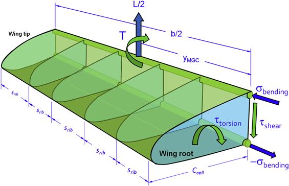
Components such as wings, fuselage, HT, VT, and control surfaces frequently require direct weight estimation. Nowadays, access to solid modeling software simplifies the effort considerably and can become fairly accurate (but remember: garbage in – garbage out!). However, if one doesn’t have access to such software, one must resort to weight modeling via geometric analysis. The quality of effort is dependent on the analyst. An example of how such estimation is detailed in this section, using a simplified representation of a wing, whose total lift is denoted by L. It can be easily extended to quickly assess material requirements for other lifting surfaces as well.
6.5.1 Direct Weight Estimation for a Wing
It is important to recognize that this method is just intended to get you “in the ballpark.” It is not a substitute for a detailed load and structural analysis. It will not consider other failure modes (buckling, crippling, etc.) and loading (asymmetric, deflected controls, etc.). Also, a single-cell torsion box structure is assumed, but a more refined version of this method could assume more than one spar (multi-cell).
Note that for initial design purposes it is common to break the wing structure into categories based on structural role:
Consider the simple wing of Figure 6-6, whose top view is shown in Figure 6-7. Such a wing, if made from aluminum, would typically feature a main spar, aft spar (or shear web), ribs, and skin riveted together to form a stiff but light structure. Note that although the following discusses wings in particular, the method applies for any lifting surface that features spars, ribs, and skins, such as horizontal and vertical tails.
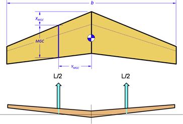
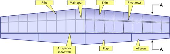
Figure 6-8 shows an arbitrary cross section of the wing. The upper image shows the extent of the control surface (e.g. flaps or aileron), while the lower shows structural detail inside it.
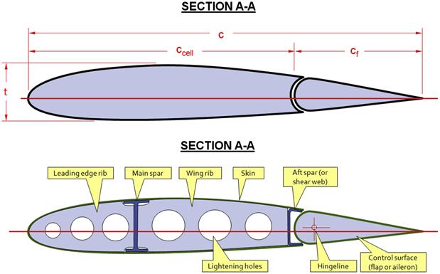
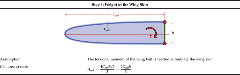
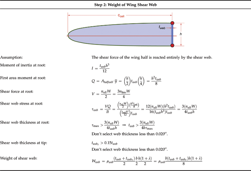
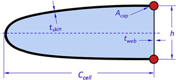
In order to allow a rapid estimate of the weight of the wing, the structure is idealized. This is shown in Figure 6-9. The entire cross-sectional area of all spar caps2 is concentrated in the upper and lower spar caps. If multiple spars are used, the average height of the spars should be used to avoid overestimation of the structural depth. Similarly, the entire thickness of all shear webs is concentrated in the idealized shear web. A idealization takes place by assuming the skin and airfoil to be represented by a parabolic D-cell section as shown in the figure. It will be assumed that spacing between ribs is one-half the average cell length and that their thickness equals that of the skin. There are limitations to this idealization that the designer should be aware of. These include the omission of electrical harnesses; fuel and control system; and hard-points for landing gear or external ordnance.

The critical loads reacted by the structure must be identified before the weight can be calculated. The designer must know the expected ultimate load factor the airplane will be designed to, as well as a representative candidate airfoil. The airfoil is necessary so we can calculate the torsion to be reacted. If the torsion with flaps deflected exceeds that at dive speed, it must be used. The critical loads are then applied to the wing as shown in Figure 6-10. If the design gross weight of the aircraft is denoted by W0, the maximum lift of the airplane, L, will depend on the ultimate load factor as follows:
![]() (6-47)
(6-47)
If we ignore the fact that a part of this lift will be carried by the fuselage and horizontal tail, this assumes the wing reacts the entire lift. Each wing, thus, reacts one-half of that total force and torsion, T, both of which are calculated as follows:
![]() (6-48)
(6-48)
The method below assumes these to be applied to the wing, as shown in Figure 6-10. The lift force must be applied at the spanwise location of the mean geometric chord to ensure the bending moment is accounted for and reacted in the spar caps. Since the lift and torsion are really distributed loads and not a point load and moment as indicated in Figure 6-10, both are zero at the wingtip and reach the maximum at the wing root, as approximated by Equation (6-48). For this reason we will allow the geometry of the structure to taper to a certain minimum value, as it would in a real wing. Otherwise, we will greatly overestimate the weight of the structure. A suitable spar cap area, Acap, at the tip can be assumed to be 5–10% of the area at the root. The wing skin and shear web can be assumed to gradually reduce to the minimum aluminum sheet thickness 0.020′′.
Note that compression strength is picked rather than tensile strength to be conservative. See the list of variables for definitions of terms.


EXAMPLE 6-4
Estimate the wing weight for a light airplane of Example (6-3) with the following specifications:
Cm = average airfoil pitching moment = -0.1
L = wing sweep at 25% MAC = 0°
NZ = ultimate load factor = 1.5 × 4.0 = 6.0g
S = trapezoidal wing area = 130 ft2
t/c = wing thickness to chord ratio = 0.16
Aluminum sheets are available in the following thicknesses:
Compare this with the result of Example (6-3). Assume the wing main element chord is 70% of wing chord. Assume an ultimate shear strength of 38,000 psi and ultimate compression strength of 44,000 psi. Assume constant material thickness for the entire wing and select thicknesses from the Available Thickness table. ρ2024 = 0.1 lbf/in3.
Solution
Step 3: Determine Structural Geometry at the Root and Tip
Note that the subscript “R” stands for root and “T” for tip.
Step 4: Determine Skin Thickness
This is the skin thickness required at root.
Using the Available Thickness table the minimum sheet thickness larger than this value is 0.016′′. However, we will select the larger recommended minimum of 0.020′′ thickness and this is also the thickness at the tip of the wing half.

Step 6: Determine Shear Web Thickness
We will thus select a web thickness of 0.025′′ for the root area and 0.020′′ for the tip area.
Step 8: Determine Spar Cap Area
This is the axial force (or force couple) in the spar caps at the root of the wing.
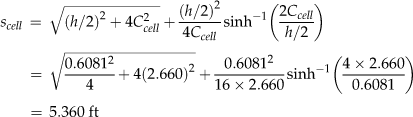
Step 12: Determine Wing Weight
The weight of this wing is significantly less than the result of Example 6-3. The reason is that this only represents the weight of the main wing element. It omits control surfaces, their attachment hard points, wing attachments, control system, fuel system, electric system, wingtip fairing and so on. The ratio between the two is 273/152 = 1.80. There is no guarantee this ratio is maintained for other configurations.
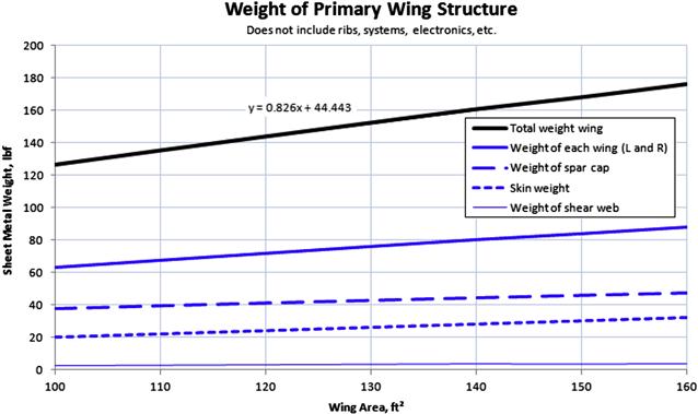
Note
It is of interest to consider how the weight of these components varies with wing area. Such a plot is shown in Figure 6-12. Such graphs come in handy when doing trade studies to evaluate an airplane’s weight as a function of wing area (see Chapter 5).
6.5.2 Variation of Weight with AR
The impact of the aspect ratio on the weight of the wing is of utmost importance in the design of the aircraft. Many designs must meet strict range or endurance requirements that call for a high-AR wing. However, it is easy to overlook that the cost of such wings is extra weight required by the high AR. At other times, the designer may want to evaluate the impact of an AR change of a mature design, or even an existing aircraft. This section presents an approximation for the evaluation of such changes.
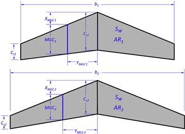
Consider the special case for which the wing area, S, and taper ratio, λ, are constant, but the AR is allowed to vary (see Figure 6-14). Assume we have a baseline wing and want to compare it to a modified wing with the same S and λ; the only change is in the AR (and therefore the dimensions of the root and tip chord). The weight of the modified AR wing can be approximated by the following assumption:
(1) There is no change in wing’s airfoil. This means the thickness ratio is constant. As a consequence, given a constant S, a higher AR results in a “thinner” wing whose chords are also shortened.
(2) It is assumed that changes in geometry are “small” enough so that change in the wing skin shear stress can be ignored. The skin shear stresses are caused by the wing torsion due to the airfoil’s pitching moment and torsion due to forward- or aft-swept wings. A large wing chord will have a greater cross-sectional area to react this torsion than a smaller wing chord, but the smaller chord wing will also generate lower pitching moments. It is prudent for the designer to evaluate whether this assumption is valid for the particular wing, but here it will be assumed the change in shear stresses are small enough to permit the same skin thickness to be maintained.
(3) It is assumed the change in AR does not require a change in other geometry that would cause components other than the wing weight to change (e.g. empennage geometry, etc.).
(4) It is assumed that there is no change in vertical shear. Therefore, the shear web thickness does not change. This is justified on the basis that changing the AR will not alter the airplane’s gross weight, only its empty weight.
(5) The maximum bending moment at the root is directly related to the location of the center of lift, which is assumed to act at the spanwise station for the MGC.
(6) The change in bending stresses is equal to the change in the bending moments. If the bending moments change by 25%, then so will the bending stresses.
(7) The change in material geometry required to react the bending moment is directly related to the change in stress levels – and therefore it is assumed the goal is to maintain similar stress levels in the spar caps before and after change.
(8) The material allowable, σmax, is assumed the same for both wing geometries.
(9) Assume the structural depth of an airfoil to be based on its maximum thickness (see Figure 6-13).
(10) Assume the spar caps have a circular cross section, separated by the structural depth (see Figure 6-13).
(11) Assume the cross-sectional area of the spar cap at tip to be 10% of that of the root.

From these assumptions it can be seen that the only change is in the dimensions of the spar caps. This implies that the only change in the weight of the structure will be associated with the change in the spar caps geometry. To estimate the magnitude of this change we begin by establishing relationships between geometry and stress.
Baseline Definitions for a Trapezoidal Wing
The following expressions are needed to begin the weight estimation and are all based on the parameters S, AR, and λ. For instance, they can be used to calculate the properties of the baseline wing.
where
Acap = cross-sectional area of the upper or lower spar cap in m2 or ft2
nult = ultimate flight load in gs.
W = airplane design gross weight in N or lbf
ρcap = weight density of spar cap material in N/m3 or lbf/ft3
σmax = tensile stress allowable of spar cap material in Pa or lbf/ft2
With respect to the ultimate flight load, nult, the load must be the maneuvering or gust load, whichever is larger. Note that many of the derivations below refer to equations in Chapter 7, The wing planform.
Derivation of Equation (6-50)
Insert Equation (6-6) into Equation (9-8) to determine the location of the center of lift:
![]()
QED
Derivation of Equation (6-51)
Consider Figure 6-13, which defines the structural depth of the airfoil, h. At the MGC this depth is given by:
![]()
Then, insert Equation (9-20) and manipulate algebraically:
![]()
QED
Derivation of Equation (6-52)
The maximum bending moment is given by3:
![]()
where L is the lift, nult is the ultimate load factor, and W is the weight of the airplane. Inserting Equation (6-50) for yMGC yields:
![]()
QED
Derivation of Equation (6-53)
The moment of inertia can be calculated from the parallel-axis theorem, assuming the spar caps have an area Acap and are separated by the structural depth h:
![]()
Inserting Equation (6-51) for structural height yields:
![]()
Finally, yielding:

QED
Derivation of Equation (6-54)
Maximum stress at the outer fibers may not exceed:
![]()
We can use this expression to determine the minimum area Acap required for the spar caps.
![]()
Inserting the proper relations for Mmax and h:

QED
Derivation of Equation (6-55)
The total volume of spar caps, assuming the thickness at the tip is 10% of that at the root:
![]()
The spar cap weight is thus:
![]()
QED
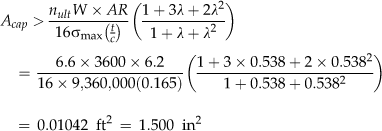
EXAMPLE 6-5
Let’s evaluate how accurate these expressions are by comparing them to an existing aircraft, the Beech Bonanza A36. The Bonanza’s design gross weight is 3600 lbf, wing area 181 ft2, AR is 6.2, and λ is 0.538. The Bonanza’s airfoils are the NACA 23016.5 at the root (t/c = 0.165) and 23012 at the tip (t/c = 0.12). Use the root thickness ratio, 0.165, for the variable t/c. The airplane is certified under 14 CFR, Part 23, in the utility category. This means the ultimate load factor is 4.4g × 1.5 = 6.6g. Assume the spar caps are fabricated from 2024-T3 extrusion, whose density is 0.1 lbf/in3 and σmax = 65,000 psi (or 9,360,000 psf). Evaluate the above parameters based on these numbers and compare to values that are in the public domain.
Solution
![]()
![]()
Spanwise location of the center of lift:
![]()
![]()
Maximum bending moment at the plane of symmetry:
![]()
Required maximum spar cap area at the plane of symmetry:
Moment of inertia at the plane of symmetry:
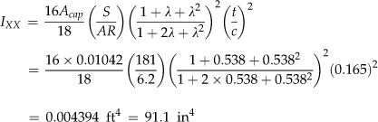
![]()
Comparison of the approximated to official numbers are shown in Table 6-2 below:
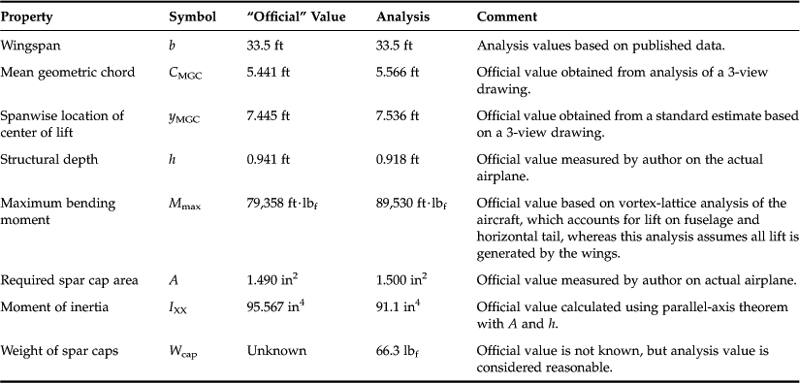
These results show this method is in good agreement with the “official” values, and lends support to its validity.
Method of Fractions
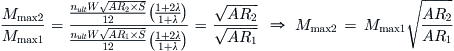
Once the baseline properties are known, we can now estimate the properties of a modified wing whose only geometric change is the AR (S and λ are assumed constant for both). Assume we have defined a baseline configuration, denoted by the subscript 1, and a comparison configuration, denoted by the subscript 2. Then, the following ratios hold between the two wings.
Derivation of Equation (6-57)
Using Equation (6-49) and applying the proper subscripts then dividing one MGC by the other leads to:
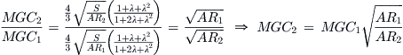
QED
Derivation of Equation (6-58)
Using Equation (6-50) and applying the proper subscripts and dividing one yMGC by the other leads to:

QED
Derivation of Equation (6-59)
Using Equation (6-51) and applying the proper subscripts and dividing one h by the other leads to:
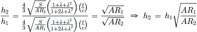
QED
Derivation of Equation (6-60)
Using Equation (6-52) and applying the proper subscripts and dividing one Mmax by the other leads to:
QED
Derivation of Equation (6-61)
Using Equation (6-54) and applying the proper subscripts and dividing one IXX by the other leads to:
QED
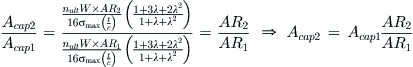
Derivation of Equation (6-62)
Using Equation (6-18) and applying the proper subscripts and dividing one IXX by the other leads to:
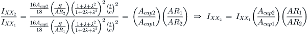
Now, let’s insert Equation (6-61) and simplify:
![]()
QED
Derivation of Equation (6-63)
Maximum stress at the outer fibers may not exceed:
![]()
Now, let’s insert Equation (6-61) and simplify:
![]()
QED
EXAMPLE 6-6
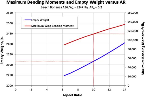
Use the method of fraction to estimate the change in empty weight for the Beech Bonanza A36 aircraft of Example 6-5, for AR increasing from 6.2 to 14. This assumes the only change is in the weight of the spar caps. The standard empty weight is 2247 lbf. Plot the change in empty weight and maximum bending moments.
Solution
All baseline values are calculated in Example 6-5, including the estimated baseline weight for the spar caps of 66.3 lbf and maximum baseline bending moment is 89530 ft·lbf. The baseline AR1 is 6.2. Let’s calculate a sample value using AR2 = 10.
Maximum bending moment for AR2 = 10:
![]()
In order to estimate the empty weight we first compute the spar cap weight for AR2 = 10 and then use Equation (6-29) to determine the difference between the two. We then add this difference to the baseline empty weight.
![]()
Therefore, the difference is:
![]()
The empty weight is therefore:
![]()
The remaining values are plotted in Figure 6-15, which shows how AR can affect aircraft weight.
6.6 Inertia Properties
The determination of various inertia properties is imperative during the design process. Properties such as moments and products of inertia are required to predict dynamic stability, and, thus, play a major role in the development of the OML. Table 6-3 lists a number of required inertia properties need for such analyses. In this book, the term “at a specific condition” refers to some particular atmospheric conditions or a specific event during a flight, for instance the end of cruise or the start of descent. During the design stage, inertia properties are considered at many such specific events. They differ from the properties at take-off, as fuel would have been consumed, or external stores dropped (for military aircraft). Fuel for jets usually constitutes as much as 20% of their T-O weight, and some 10–15% for piston engines. Therefore, there can be a large change in the inertia properties between T-O and landing, and this can have a profound effect on dynamic stability.
TABLE 6-3
| Property | Symbol | Section |
| Weight at a specific condition | Wtot | 6.6.3 |
| Center of gravity (CG) in terms of location | XCG, YCG, ZCG | 6.6.5 |
| CG is also given in terms of %MAC (in particular XCG) | XCG | 6.6.5 |
| Moment of inertia about the x-, y-, and z-axes | IXX, IYY, IZZ | 6.6.7 |
| Product of inertia in the xy-, xz-, and yz-planes | IXY, IXZ, IYZ | 6.6.7 |
6.6.1 Fundamentals
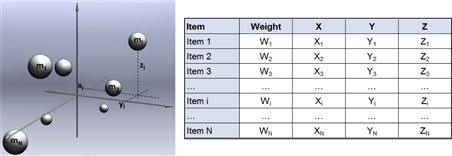
The process of determining inertia properties typically involves treating components as a collection of point loads; i.e. as a weight and position in space (see Figure 6-16). This allows properties such as the weight, or moments and products of inertia of the vehicle to be estimated using the methods to be introduced shortly. Then, the inertia properties for the entire collection are determined by a simple summation. The moments and products of inertia of large objects, such as wings, and heavy objects, such as engines, should be included in the total for further accuracy and this is indicated in the formulation that follows. Depending on the location and shape of such components, the moments and products of inertia of the parts themselves can easily add 25%, and even higher values, to the total amount calculated by the parallel-axis theorem.
In this section, the inertia properties shown in Table 6-3 will be calculated.
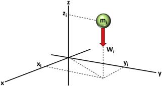
The formulation presented in this section assumes the airplane can be represented by a collection of point loads in three-dimensional space, as shown in Figure 6-17. Note that each arbitrary point is denoted by the subscript i.
6.6.2 Reference Locations
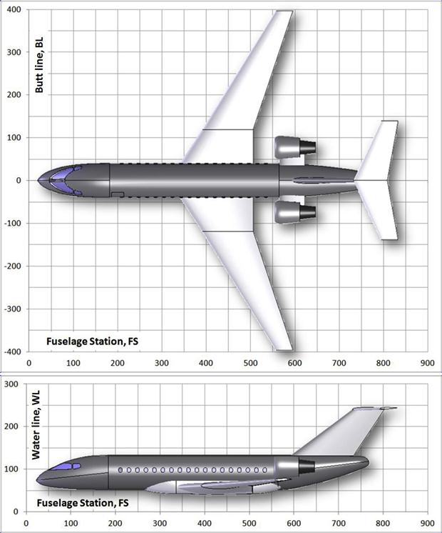
The aerospace engineer should use terminology commonly used in the aviation industry when referring to a point in space at which a specific weight is located near an aircraft. For instance, consider the location of avionics equipment or an occupant. The physical location is referred to using terms such as:
| FS – fuselage station | BL – butt (or buttock) line |
| WL – water line | WS – wing station |
| HS – horizontal station | VS – vertical station |
FS, BL, and WL, are depicted in Figure 6-18. When an airplane features swept wings or tail, it is convenient to represent locations using a wing, horizontal, or vertical station. These are effectively a BL aligned to something like the quarter-chord line or another conveniently selected datum.
EXAMPLE 6-7
The CG of an airplane is reported to be at FS191.3 (in other words: at fuselage station 191.3 inches). If the LE of the MGC airfoil is at FS185 and the MGC is 6.32 ft, where is the CG with respect to the MGC?
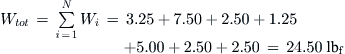
6.6.3 Total Weight
As applied to an airplane, we break it into a finite number of subcomponents: engine, propeller, left wing, right wing, horizontal tail, fuselage, left main landing gear, right main gear, and so on, whose weights we can assess. These are denoted by Wi, where the index i is assigned to each component. Then, the total weight of the collection of components is calculated as follows:
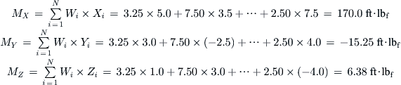
6.6.4 Moment About (X0, Y0, Z0)
Moments about an arbitrary reference point (X0, Y0, Z0) are calculated using the expressions below. This is a necessary intermediary step before the center of gravity (CG) can be calculated:
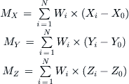 (6-66)
Unless otherwise specified, our reference point is always (0, 0, 0) and this is assumed in the following formulation. We rewrite Equation (6-66) by writing the moments about the point (0, 0, 0):
![]() (6-67)
(6-67)
6.6.5 Center of Mass, Center of Gravity
Consider a system of matter (this could be a collection of solid objects, liquids, gases, or any combination thereof) distributed in three-dimensional space. Then, we define the center of mass (CM) of the system as the point in space at which uniform force acting on the whole system is equivalent to that force acting at just that point.
In a uniform gravitational field, the force acting on the system can be considered to act at the CM, in which case we refer to it as the center of gravity (CG). While the CM and CG are often used interchangeably, this does not hold true in non-uniform acceleration fields. However, in the context of this book, it is always assumed the airplane is operated in a uniform acceleration field and, therefore, the CM and CG are always the same point. The position of the CM, R = (XCM, YCM, ZCM), can be calculated from:
![]() (6-68)
(6-68)
where
Similarly, the location of the center of gravity of the collection of components is estimated using the following expressions:
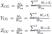 (6-69)
It is very common to present the X-location of the CG in terms of %MAC (although it really refers to MGC). This would be calculated as follows, where XMGC is a reference distance to the leading edge of the MGC, although this is shown to reference the apex of the swept back wing in Figure 6-19:
![]() (6-70)
(6-70)
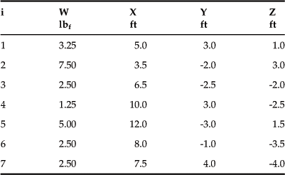
EXAMPLE 6-8
The following collection of point loads is given in Table 6-4. Determine the total weight, moments, and the location of the CG in 3-dimensional space.

6.6.6 Determination of CG Location by Aircraft Weighing
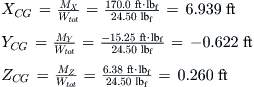
The CG location of actual aircraft is always determined by direct weighing. Small aircraft are parked on specially designed weighing kits, which consist of three separate electronic scales; one for the nose gear and two for the main gear (see Figure 6-20). A special device simultaneously connects to all three, allowing the weight on each wheel and the total to be read. Larger aircraft are often equipped with special jacking points used for the same purpose. The advantage of such hardpoints is that their spatial location is known. This contrasts with many fixed landing gear configurations, whose measurements are affected by structural flex, which introduces inaccuracy. Then, once the distance between the weighing points is known, the measured weights can be used to calculate the location of the CG as shown below:
where
RM = main gear reaction, the sum of both main gear scales
W = total aircraft weight = RN + RM
xN, xM, and xNM = distances defined in Figure 6-20
Note that the CG location is usually determined with respect to some datum. However, this differs among airplane types. The above expression is generic and by locating the nose landing gear with respect to such a datum the CG can be represented in terms convenient to the designer or operator. Additional methodologies are provided by D’Estout [7]. Note that when weighing an aircraft in this fashion, it is imperative that it is leveled as accurately as possible and that no wind conditions prevail where the weighing takes place.
6.6.7 Mass Moments and Products of Inertia
Fundamental Relationships
Any object that rotates about some axis has a tendency to continue that motion, just like an object moving along a straight path has a tendency to move along that path. The former is an example of rotational momentum (think of a flywheel) and the latter of linear momentum. Unless acted on by some force, both will continue this motion indefinitely. The tendency of a rotating body to continue its motion depends on two properties: its mass and the distance of its CG from the axis of rotation. This leads to the definition of mass moment of inertia as the property of an object that is to rotational momentum what mass is to linear momentum.
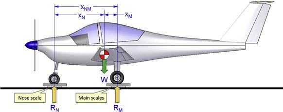
The moment of inertia of a point mass, m, with respect to such an axis is defined as the object’s mass times its distance, r, from the axis squared (see Figure 6-21). Mathematically, the moment of inertia of the mass about point O is given by:
![]() (6-73)
(6-73)
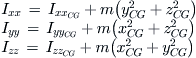
where W is the weight of the object and g is acceleration due to gravity. In aircraft stability and control theory we are primarily interested in evaluating the moment of inertia about the x-, y-, and z-axes. Therefore, Equation (6-70) must be evaluated for each axis and the results would be presented as follows:
![]() (6-74)
(6-74)
The mass moment of inertia of an arbitrary body of constant density and continuous mass distribution can be determined by integrating the contribution of the infinitesimal mass, dm, over the volume of the body about an arbitrary axis of rotation, O (see Figure 6-22):
![]() (6-75)
(6-75)
where B is used to indicate the integration is performed over the entire body. This way, the moment of inertia about an axis is a measure of the distribution of matter about that axis. As stated earlier, aircraft stability and control theory requires the moments of inertia to be determined about three mutually orthogonal axes that go through the CG. Equation (6-75) is then rewritten accordingly for each axis by noting that r2 about the x-axis is given by (y2 + z2), r2 about the y-axis is given by (x2 + z2), and so on. Therefore, the moment of inertia about the point O is given by:
![]() (6-76)
(6-76)
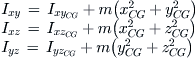
where the double-subscripts refer to a rotation about the axis indicated. The value of the moment of inertia is always positive. Note that the three orthogonal vectors that form the coordinate system about which the body rotates necessarily form three separate and mutually orthogonal planes; the xy-, xz-, and yz-planes. Rotational motion in three-dimensional space is strongly affected by how uniformly (or symmetrically) the body is distributed on each side of these planes. This inertia property is called the products of inertia and is determined as follows:
![]() (6-77)
(6-77)

The value of the product of inertia can be negative or positive. The products of inertia are a measure of the symmetry of the object. An airplane is often symmetrical about one of the planes – the xz-plane for a standard coordinate system. For this reason, this plane is often called the plane of symmetry. The product of inertia about the xz-plane is often taken to be 0; however, this is false if the airplane has asymmetric mass loading, such as unbalanced fuel in the wing tanks, or a single pilot in a two-seat, side-by-side, cabin. Considering Ixz = 0 for such an asymmetric loading can only be justified if its magnitude is negligible compared to the other moments and products of inertia. It is not justifiable if one wing fuel tank is full and the other is empty.
Parallel-axis Theorem for Moments of Inertia
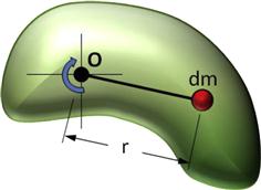
Consider Figure 6-23, which shows an arbitrary body rotating about a point other than its CG. The distance between the CG and the axis of rotation, O, is denoted by rCG. The distance from the axis of rotation to the infinitesimal mass dm is given by r and the distance between it and the CG is given by r′. If the moment of inertia must be evaluated for this situation, evaluating Equation (6-76) leads to a convenient theorem in which the moment of inertia is given by the following expression
![]() (6-78)
(6-78)
where
ICG = moment of inertia of the body about its own CG.
r′ = distance from CG to an infinitesimal mass dm
rCG = distance from the reference point O to the CG of the body
Equation (6-78) is referred to as the parallel-axis theorem. A more practical form of it is shown below:
 (6-79)
where
Derivation of Equation (6-78)
The moment of inertia about the arbitrary point in Figure 6-23:
![]()
Since rCG is a constant, we can simplify this and write:
![]()
By inspection, the first term represents the moment of inertia of the mass, acting as a point mass, as it rotates about point O and this is given by (remember that rCG is constant):
![]()
where the subscript P denotes the parallel axis term. The second term is zero, because the origin of r′ is at the CG, but the mass is distributed about the CG. To better see this, consider the coordinate system superimposed on the CG in Figure 6-23. The contribution of the mass lying above the x-axis will be cancelled by equal mass that lies below it. In fact, the integral is effectively a moment integral analogous to Equation (6-66), where X0 is the xCG. Finally, the third term is the moment of inertia of the body about its own CG and is given by:
![]()
From which we can write:
![]()
QED
Parallel-plane Theorem for Products of Inertia
The parallel-axis theorem can be extended to the product of inertia in a similar fashion, in which case it is referred to as the parallel-plane theorem.
 (6-80)
where
![]() moment of inertia of the body about its own CG
moment of inertia of the body about its own CG
xCG, yCG, zCG = distance from the reference point O to the CG of the body
The derivation is similar to that of the parallel-axis theorem.
6.6.8 Moment of Inertia of a System of Discrete Point Loads
The form of the moment of inertia most helpful for our analysis of the airplane is when they are written in terms of a collection of discrete mass points, similar to the treatment in Section 6.6.5, Center of mass, center of gravity. Thus we write the moments of inertia of a system of discrete point loads as follows:
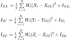 (6-81)
Note that the terms involving the product of the weight and distance from the CG represent the application of the parallel-axis theorem. The last term of each equation is the moment of inertia of the body itself. For instance, a typical piston engine can have a significant moment of inertia about its own CG and this should be included in the estimation. However, the moment of inertia of some particular piece of avionics about its own CG is usually negligible and may be omitted.
6.6.9 Product of Inertia of a System of Discrete Point Loads
The product of inertia is estimated in a similar fashion as the moments of inertia, although added care must be exercised, as the position of a component on either side of each plane must be included with the proper sign.
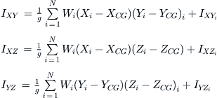 (6-82)
where
6.6.10 Inertia Matrix
The moments and products of inertia about a specific point are often represented in a matrix format, as this lends itself conveniently for various dynamic stability analyses. This matrix is called the inertia matrix and it is always symmetric. Here, it is shown in a format that assumes the axes of interest of go through the airplane’s CG.
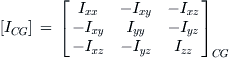 (6-83)
The inertia matrix is dependent on the orientation of the axes going through the CG. One particular orientation results in the matrix becoming diagonal. The axes that cause this special form are called the principal axes of the matrix. The principal axes are dependent on the location of the reference point; shifting the reference point to a new location will change the orientation of the principal axes.
6.6.11 Center of Gravity Envelope
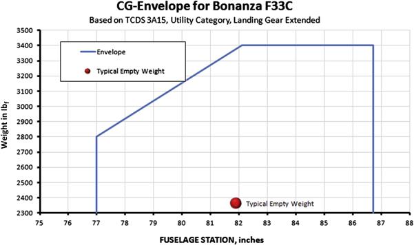
Currently, aviation regulations dictate that all aircraft certified as GA aircraft (14 CFR Part 23) must be statically stable and, dynamically, the Dutch roll mode must be stable, while spiral stability and phugoid modes may be slightly divergent. This implies the CG of the aircraft must remain in the neighborhood of a specific location in space, with respect to the airplane, throughout the duration of any flight. This neighborhood is called the center of gravity envelope, or simply, a CG envelope (see Figure 6-24). The location of the CG is of paramount importance to the pilot of an airplane and it is his or her responsibility to ensure the aircraft is loaded such that the CG remains inside the allowable envelope throughout the entire duration of the flight.
Design Guidelines
In the interests of safety, the reference point (0, 0, 0) to which the CG refers is usually placed far in front of and below the nose of the aircraft. This ensures that when moments due to the positions of discrete weights are being calculated, all the spatial locations only have a positive sign and not a combination of positive and negative signs. This reduces the chance of mathematical error creeping into calculations, and, therefore, the chance of erroneous results that might indicate the CG was inside the CG envelope, when in fact it was outside it.
There are two common ways to indicate the location of the CG for GA aircraft. The first presents it in terms of percentage of the mean geometric chord. The second expresses it more explicitly in terms of the fuselage station (FS). The use of each differs between aircraft manufacturers. The design engineer should be familiar with both methods.
The CG envelope in Figure 6-24 is based on the Type Certification Data Sheet (TCDS 3A15 [8]) for the Beech F33C Bonanza and shows the location of the CG may vary from fuselage station 77, or FS77 to FS86.7 up to 2800 lbf, but from FS82.1 to FS86.7 at 3400 lbf. The FS are in units of inches. Additionally, the plot shows the CG location and weight for a typical empty F33C Bonanza aircraft.
6.6.12 Creating the CG Envelope
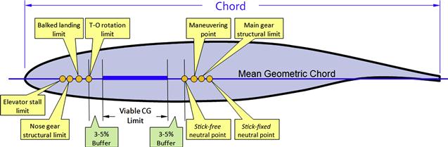
The aforementioned section shows that the creation of the CG envelope is a crucial and necessary step. Its goal is to determine how far forward and aft the CG may travel without compromising the safe operation of the aircraft. Unfortunately, this is not as simple as that, as these limits may depend on aerodynamic (i.e. stability and control) and structural issues. Figure 6-25 shows parameters that are typically considered when determining a viable CG envelope. Note that the order of the critical CG locations may be transposed. Also, other considerations may apply to your particular aircraft design that are not reflected here. Ultimately, it is the responsibility of the design leader to ensure that a viable CG envelope has been established. The safe operation of the airplane depends on this task being accomplished correctly.
In the opinion of this author, the designers of selected kit planes have done a less than acceptable job at this and designed airplanes that operate with the CG too far aft. This manifests itself in airplanes with very light stick forces and requires piloting more like what one would expect from a marginally stable aircraft. This may have been done under the pretense that it makes the airplane more “responsive” and “fun to fly,” but a more plausible explanation is that it stems from the designer’s lack of understanding of stability and control theory. For instance, an airplane that the pilot is advised to handle with care because “it is so easy to start a PIO”4 is an airplane with unacceptable longitudinal characteristics. Such airplanes are dangerous, no matter how “fun to fly.” The customers of such airplanes are often unaware of the risks involved in flying such airplanes and sometimes pay dearly. Make sure you don’t fall into this trap.
Determination of the Aft CG Limit
The first step in determining a viable CG envelope lies in the determination of the so-called stick-fixed neutral point. The name comes from the fact that it assumes the elevator is immovable, typically in the neutral position. This point is generally a good indicator of how far aft the CG can go, but is not the final answer. There are at least two other points that must also be determined and have to do with stability and control; the stick-free neutral point and maneuvering point. The former requires knowledge of the elevator hinge moment and the latter about the pitch damping characteristics of the airplane. Each of these points will yield a maximum value for the CG location beyond which the aft CG may not cross. Furthermore, for a conventional tricycle landing gear, the structural capabilities of the main landing gear should also be accounted for. If the CG moves too far aft, the main landing gear reaction loads increase and can eventually lead to structural failure (the same holds for the nose landing gear if the CG is too far forward). The landing gear or airframe design teams typically furnish the aerodynamicist with this information.
Determination of the Forward CG Limit
Characteristics that affect the forward points are also shown in Figure 6-25 and Figure 6-26. The elevator stall limit indicates where the maximum deflection of the elevator has been reached and the lift coefficient required to trim the airplane would cause one of the following two scenarios: the elevator stalls, which means there is no additional elevator authority remaining; or the lift coefficient required by the horizontal tail (with the elevator fully deflected trailing edge up) is so high it implies it has exceeded its stall AOA. Generally, rather than allowing the controls to reach such extremes, the experienced aerodynamicist places a limit on each (see Section 23.3, GA aircraft design checklist).

A balked landing limit represents a condition in which the pilot of an airplane, in the landing configuration, aborts the landing procedure for a go-around. This is a very demanding situation for the airplane because it is flying slowly, with flaps fully deployed, and at full power. This limit is similar to the elevator stall limit in the sense it represents a demand for too large an elevator deflection. The T-O rotation limit results from the elevator being unable to lift the nose gear off the ground during the T-O run.
These limiting CG locations cited above fall around the viable CG envelope and dictate the usable limit. Some limits, such as the landing gear structural limits or the elevator limits, are typically presented as isobars (see Figure 6-26). The structural isobars are determined during the detailed design phase. The elevator limit isobar is determined using stability and control theory. The figure shows how the three isobars affect the shape of the envelope in different ways. The NLG isobar dictates the forward light limit (here 10% MGC at 2800 lbf). The elevator limit isobar forces the forward limit at 3400 lbf at 17% MGC) and the MLG isobar forces the aerodynamicist to move the aft envelope line farther forward (sloping it in the process), even though the airplane might be quite capable of being more aft. With respect to Figure 6-25, the viable envelope should generally offer between 3% and 5% MAC buffer, forward and aft of the corresponding limiting points, in case there are analysis inaccuracies.
Loading Cloud
The generation of a loading cloud is an important step that should be completed for any aircraft that carries more than one occupant. It is a graph showing the CG envelope and as many combinations of occupants, baggage, and fuel as is practical. An example of this is shown in Figure 6-27, constructed using the data of Table 6-5. The plot gives a lot of clues about the range of weights and CG locations the airplane must operate within and whether it is likely to be operated outside the proposed CG limits. An airplane that requires the operator to constantly worry about whether it is loaded outside the CG limits is one that is likely to accrue criticism. As such, the loading cloud is helpful during both the preliminary stage and development of production vehicles.
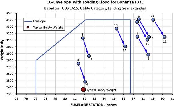
FIGURE 6-27 Example of a loading cloud. It exposes a serious problem, here destined to render the aircraft “illegal” for a careless pilot. If this happens to your aircraft and the load combinations are “practical” (unlike the ones shown here), then do something about it! – move the wing, move heavy parts around to place the empty weight CG in a better location, so the envelope can accommodate most of the cloud. Just do something.
TABLE 6-5
Tabulated Loading Combinations Used to Create the Loading Cloud of Figure 6-27. Note that weights are in lbf and arms in inches

As stated above, the graph is created by calculating the CG location and weight for selected combinations of occupants, baggage, and fuel weight. The basic graph of Figure 6-27 is based on the single-engine, four-seat Beechcraft F33C Bonanza aircraft and uses the calculation methodology of Section 6.6.11, Center of gravity envelope. The data calculated in Table 6-5 are superimposed to help one visualize how well the CG envelope contains the loading combinations. As can be seen, some of the combinations consist of various amounts of fuel, occupant, and baggage weights. This way, each row has its own total weight and CG location, which is plotted in Figure 6-27. The figure shows that the F33C hardly has a forward loading problem, but is easily loaded outside the aft CG limit. This results from the relative aft position of even the front seats. In defense of the F33C, some of the load combinations presented are arguably “preposterous” or “unfair.” However, they are presented to emphasize the importance of reviewing the rationale behind particular loading scenarios. For instance, considering Combo IDs 11 and 12, it is not plausible that a competent pilot would store 270 lbf in the baggage area, with an empty seat farther forward, not to mention that 270 lbf might exceed the allowable load in the baggage area.
The loading cloud reveals primarily two properties of the load combination: the most forward and aft CG location the airplane is likely to ever see in practice; and the maximum and minimum weight margin expected during operation. The importance of performing this sort of analysis cannot be overemphasized. For instance, when certifying a new airplane, the authorities will require the manufacturer to demonstrate compliance to the regulations at each extreme of the CG envelope. This means the airplane must be loaded to these extremes, and demonstrated to satisfy applicable regulations. This can lead to situations that are better avoided, as explained in the next paragraph and highlighted in Figure 6-28.
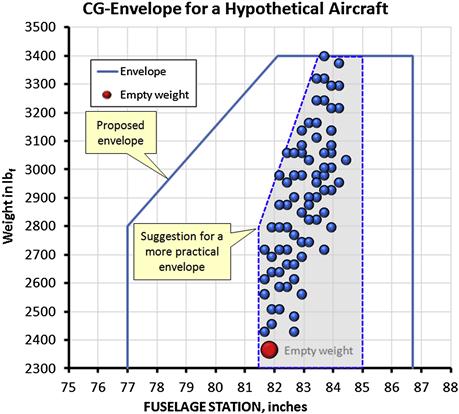
Consider a scenario that sometimes comes up in practice; too large a CG envelope. The initial CG envelope may have been based on analysis and even preliminary flight testing. However, it may be found to exceed what the airplane will ever be exposed to in operation. This may be the consequence of the loading possibilities of the aircraft; for instance due to seating arrangement (e.g. side-by-side seating), limited travel with fuel consumption, and other factors. An unnecessarily large CG envelope may bring about a serious headache for the flight test team because the airworthiness of the vehicle must be demonstrated at the extremes of the envelope. Our hypothetical aircraft would require heavy ballast to be mounted in awkward places to allow it to be flown at the extremes of the envelope. It might even require special temporary hardpoints to be designed, fabricated, and installed to carry the ballast. It is really a wasted effort, rendering it far more sensible to simply redraw a narrower envelope to resemble that of the shaded area in Figure 6-28. This will shave off certification cost and effort and the resulting airplane will be equally useful as the one featuring the wider envelope.
6.6.13 In-flight Movement of the CG
All aircraft that burn fossil fuels will reduce their weight during flight. Some aircraft will reduce their weight by other means, such as airplanes dropping parachutists, or military aircraft jettisoning empty fuel tanks or ordnance (missiles, bombs, etc.). This movement must be considered during the design phase of the aircraft, and may not cause the CG to move out of the CG envelope. Often this requires components to be relocated to ensure the airplane can contain the CG location inside the CG envelope regardless of such weight changes. Figure 6-29 shows an example of the Beech F33C Bonanza with two 200 lbf-people and full tanks of fuel (74 gals usable) as the fuel is completely consumed. This example is based on specifications given by TCDS 3A15 for the airplane. It shows that the CG moves back an inch or so but, more importantly, that the CG stays inside the airplane’s envelope.
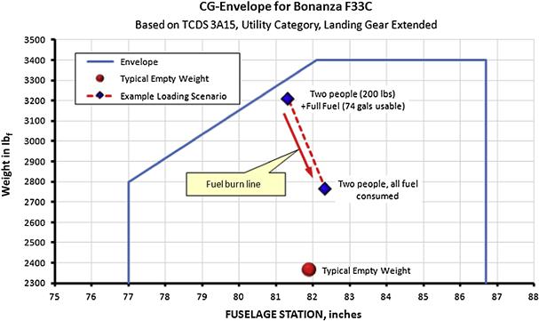
6.6.14 Weight Budgeting
The purpose of weight budgeting is to provide constraints and impetus for airframe designers to design parts with strong emphasis on weight. It is a common problem in the aviation industry that components are overdesigned, which means that parts are unnecessarily strong and, thus, too heavy. This is one of the primary reasons why empty weight targets get busted during the development of aircraft. Weight budgeting helps the weight reduction effort to stay where it belongs: with the cognizant designer (airframe, avionics, power plant, and so on).
Another important purpose is that it helps the engineer understand where effort toward weight reduction is most likely to bear fruit. This is important if empty weight targets have not been met. Remember the adage: “reducing 1000 lbs by 1% is better than reducing 1 lb by 50%.”
The weight budgeting process begins by breaking the complete aircraft into categories, such as Wings, Horizontal Tail, Vertical Tail, Fuselage, Landing Gear, Powerplant, etc. Sometimes such categories are broken down further, e.g. Wings-Left Main for the main element of the left wing, Wings-Ailerons, Wings-Flaps, Wings-Electrics, and so on. An example of a weight budget breakdown as used for weight management in the development of a prototype is shown in Table 6-6.

This example shows that the projected weight of this aircraft is some 269 lbf higher than planned. This might be acceptable for a test vehicle, although it could cause complications in a flight test program, in particular if the weight of available fuel for test flying is compromised. But it is unacceptable for the production airplane as it amounts to 10% over target.
6.6.15 Weight Tolerancing
During the preliminary design phase it is impossible to pinpoint a precise location for the CG or magnitudes of moments and products of inertia, as final weights and CG locations of individual components are constantly changing. For instance, the location of the engine’s CG may be specified as some value Xengine ± Δx. It may be an engine in development and its weight may be given as Wengine ± ΔW. As an example, the engine manufacturer might specify the weight of the engine to be 356 ± 15 lbf. Consequently, the moment contribution of this engine to the total moment about the reference point (0, 0, 0) would be a range along the x-axis, rather than a specific point, computed as follows:
![]() (6-84)
(6-84)
Under such circumstances it is better to consider these as a “sphere” of possible values, rather than a single specific point. In the process, the designer can assess the probability of the CG being outside the allowable limits. This section develops equations that allow the aircraft designer to keep track of these important parameters by assigning tolerances to them.
Consider a collection of point loads positioned in three-dimensional space whose weight and position are known to a certain level of accuracy (tolerance) only (see Table 6-7). Then, the inertia properties for such a collection are defined as follows:
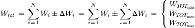 (6-85)
X-moments about the point (0, 0, 0):
 (6-86)
Y-moments about the point (0, 0, 0):
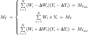 (6-87)
Z-moments about the point (0, 0, 0):
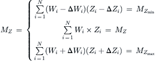 (6-88)
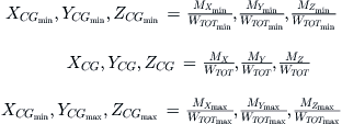 (6-89)
EXAMPLE 6-9
A collection of point loads is given in Table 6-8. Determine a probable location of the CG along the x-axis by accounting for tolerances.

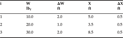
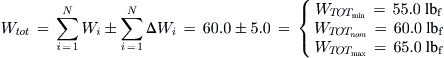
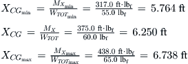
where
Exercises
(1) Determine the useful load, empty weight ratio, and fuel weight ratio for an airplane whose gross weight is 1650 lbf, empty weight is 950 lbf, and which can carry 33 gallons of avgas.
(2) You have been asked to design a twin-engine, piston-powered GA aircraft that requires only one pilot for operation. The customer wants the airplane capable of taking off at the design gross weight with a useful load that consists of eight 200 lbf-individuals (which includes the pilot), 200 gallons of avgas and 350 lbf of baggage on board. Additionally, he or she wants the design’s empty weight to amount to no more than 65% of gross weight. Determine the empty weight (We), gross weight (Wo), useful load (Wu), payload (Wp), crew weight (Wc), fuel weight ratio (Wf/Wo), and empty weight ratio (We/Wo). Compare the empty weight ratio to the one obtained using the formulation of Section 6.2.2, Method 2: Historical empty weight fractions, for the same class of airplanes.
(3) (a) Estimate the empty and gross weight and the corresponding CG positions using the data for the amphibious LSA aircraft depicted in Table 6-9. (b) Also estimate the airplane’s moment and products of inertia.

(4) This problem is intended to demonstrate a “typical” operational scenario for an airplane design using an actual aircraft. A CG envelope for the Beech F33C Bonanza is shown in Figure 6-24. The empty weight of the airplane is 2363 lbf and the empty weight CG location is at fuselage station (FS) 81.9 inches. The gross weight of the airplane is 3400 lbf. The airplane is to be loaded for a flight trip in accordance with the data of Table 6-10.
TABLE 6-10
Weight Data For a Hypothetical Amphibious LSA
| Item | FS, inches | Weight, lbf |
| Empty weight | 81.9 | 2363 |
| Pilot (front left seat) | 85.0 | 180 |
| Pax 1 (front right seat) | 85.0 | 140 |
| Pax 2 (aft left seat) | 121 | 200 |
| Pax 3 (aft right seat) | 121 | 120 |
| Baggage | 150 | 50 |
| Fuel | 75.0 | ? |
(a) The maximum fuel the pilot may take-off with, in lbf and US gallons.
(b) Determine the weight and FS with T-O fuel on board.
(c) Determine the weight and FS with all fuel consumed.
(d) Plot the points representing the empty weight CG, as well as those from (b) and (c).
(e) Is there a problem with the pilot’s planned loading of this airplane? If so, what is it? Is there a simple remedy he or she can apply to solve the problem? What is is? (Support with numbers where appropriate.)
(5) Consider the side view of the Cessna 177 RG Cardinal shown in Figure 6-30, as it is being weighed. This is done by placing scales under its nose wheel and the two main wheels. The airplane contains only unusable fuel and is otherwise empty. Determine the following for the airplane if the nose scale (RN) reads 275 lbf, the left main (RLEFT) reads 725 lbf, and the right main (RRIGHT) reads 695 lbf:
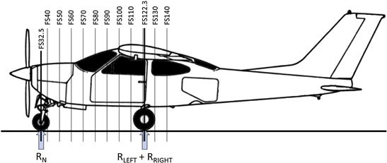
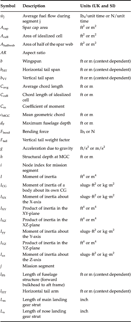

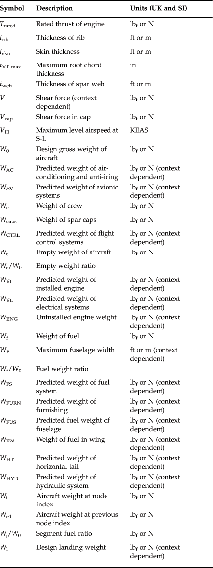
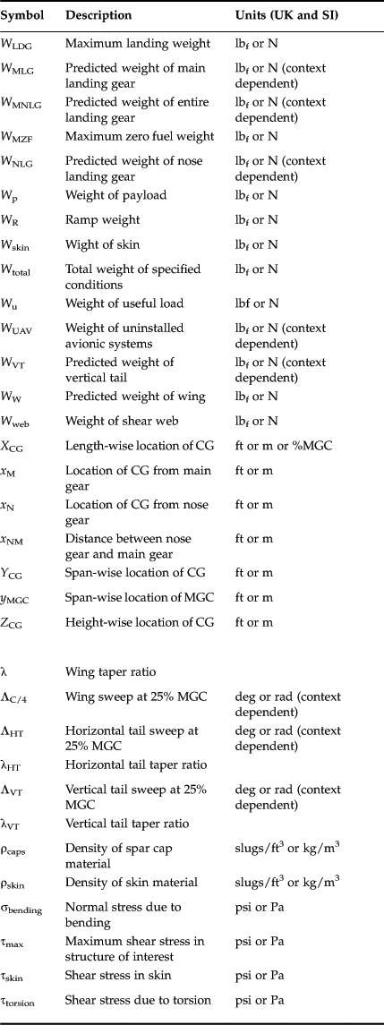
References
1. Pappalardo Joe. Weight watchers How a team of engineers and a crash diet saved the joint strike fighter. Air and Space Magazine October/November, 2006;66–73.
2. Thomas Geoffrey. Following Quantas cuts, Attention turns to 787. Air Transport World April 15, 2009.
3. Moores Victoria. Emirates seeks A380 and 747-8 Weight Control. Flightglobal October 24, 2007.
4. Raymer Daniel. Aircraft Design: A Conceptual Approach. AIAA Education Series 1996.
5. Torenbeek Egbert. Synthesis of Subsonic Aircraft Design. 3rd ed. Delft University Press 1986.
6. Nicolai Leland. Fundamentals of Aircraft and Airship Design. Volume I AIAA Education Series 2010.
7. D’Estout Henri G. Aircraft Weight and Balance Control. 4th ed. Aero Publishers 1967.
8. TCDS 3A15. Hawker Beechcraft Corporation, Revision 94, 02/25/2007. FAA.
1See for instance Section 1.3.1, Conceptual design algorithm for a general aviation aircraft.
2The term “all spars” refers to wing structures that feature multiple spars.
3Although the maximum bending moment is generally determined at the location of the wing attachments, for this method this is assumed at the plane of symmetry.
4PIO stands for pilot-induced oscillation.