The Anatomy of the Wing
Abstract
A number of methods to size the wing of a new GA aircraft are presented. The chapter begins by the presentation of handy formulation to calculate various properties of trapezoidal surfaces, which is the most common planform shape for lifting surfaces like wings and horizontal and vertical tails. This is followed by the introduction of various concepts, topics, and methods for laying out the wing planform. These include aspect ratio, taper ratio, washout, and wing incidence angle. In order to help the designer evaluate the pros and cons of typical wing planform shapes, suitable for the new aircraft, a detailed discussion follows. In addition to the large number of different geometries presented detailed information about the spanwise distribution of section lift coefficients is provided to help the designer realize their properties. Next, a number of methods to evaluate the lift and pitching moment characteristics of the wing as a 3-dimensional lifting body are provided. Then, a number of issues that have to do with wing stall characteristics and how to improve them are presented. Finally, in order to help the designer in realizing the properties of the selected wing planform and airfoils, a practical version of Prandtl’s Lifting Line Theory is presented. Despite being old, this is a sophisticated numerical method used to estimate the aerodynamic properties of the wing. A computer function, written in Visual Basic for Applications, intended for use with Microsoft Excel is presented as well, allowing the reader to get to work immediately.
Keywords
Wing planform; trapezoidal wing; reference area; aspect ratio; taper ratio; washout; washin; wing area; chord; span; section lift coefficient; angle-of-attack; angle-of-incidence; decalage; optimum lift; constant-chord (Hershey-bar); elliptic; straight-tapered; compound taper; swept; cranked; semi-tapered; schuemann; delta; double-delta; disc; lift curve; lift curve slope; maximum lift coefficient; minimum lift coefficient; zero lift angle-of-attack; linear range; design lift coefficient; law of effectiveness; flexible wings; ground effect; Oswald’s span efficiency; stall characteristics; flow separation; stall progression; Prandtl’s lifting line theory; vortex filament; Biot-Savart law; Helmholz’s vortex theorem
Outline
9.1.1 The Content of this Chapter
9.1.2 Definition of Reference Area
9.1.3 The Process of Wing Sizing
The Establishment of Basic Datum
9.2 The Trapezoidal Wing Planform
Aspect Ratio for Multi-wing Configurations
Derivation of Equations (9-6), (9-8), and (9-10)
9.2.2 Poor Man’s Determination of the MGC
9.2.3 Planform Dimensions in Terms of S, λ, and AR
9.2.4 Approximation of an Airfoil Cross-sectional Area
Derivation of Equations (9-22) and (9-23)
9.3 The Geometric Layout of the Wing
Illustrating the Difference Between Low and High AR Wings
Determining AR Based on a Desired Range
Determining AR Based on Desired Endurance
Estimating AR Based on Minimum Drag
Estimating AR for Sailplane Class Aircraft
9.3.2 Wing Taper Ratio, TR or λ
9.3.3 Leading Edge and Quarter-chord Sweep Angles, ΛLE and ΛC/4
Impact of Sweep Angle on the Critical Mach Number
Impact of Sweep Angle on the CLmax
Impact of Sweep Angle on Structural Loads
Impact of Sweep Angle on Stall Characteristics
9.3.5 Wing Twist – Washout and Washin, ϕ
A Combined Geometric and Aerodynamic Washout
Panknin and Culver Wing Twist Formulas
9.3.6 Wing Angle-of-incidence, iW
Step 1: Determine the Optimum AOA for the Fuselage
Step 2: Determine the Representative AOA at Cruise
Step 3: Determine the Recommended Wing Angle-of-incidence
Step 4: Determine the Recommended HT Angle-of-incidence
Decalage Angle for a Monoplane
9.3.7 Wing Layout Properties of Selected Aircraft
9.4.1 The Optimum Lift Distribution
9.4.2 Methods to Present Spanwise Lift Distribution
9.4.3 Constant-chord (“Hershey-bar”) Planform
9.4.5 Straight Tapered Planforms
Straight Leading or Trailing Edges
The Double-delta Planform Shape
9.4.9 Some Exotic Planform Shapes
Disc- or Circular-shaped Planform
9.5 Lift and Moment Characteristics of a 3D Wing
9.5.1 Properties of the Three-dimensional Lift Curve
Maximum and Minimum Lift Coefficients, CLmax and CLmin
Angle-of-attack at Zero Lift, αZL
Angle-of-attack where Lift Curve Becomes Non-linear, αNL
Angle-of-attack for Maximum Lift Coefficient, αstall
Angle-of-attack for Design Lift Coefficient, αC
The Relationship between Airspeed, Lift Coefficient, and Angle-of-attack
9.5.3 Determination of Lift Curve Slope, CLα, for a 3D Lifting Surface
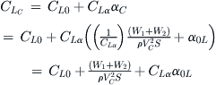
9.5.4 The Lift Curve Slope of a Complete Aircraft
Derivation of Equations (9-59) and (9-60)
9.5.5 Step-by-step: Transforming the Lift Curve from 2D to 3D
9.5.6 The Law of Effectiveness
9.5.9 Impact of CLmax and Wing Loading on Stalling Speed
9.5.10 Step-by-step: Rapid CLmax Estimation
9.5.11 Step-by-step: CLmax Estimation per USAF DATCOM Method 1
Step 1: Determine the Two-dimensional Maximum Lift Coefficient
Step 2: Plot the Distribution of Section Lift Coefficients
Step 3: Determine the AOA at which Local Cl Intersects Clmax
9.5.12 Step-by-step: CLmax Estimation per USAF DATCOM Method 2
Step 1: Determine the Taper Ratio Correction Factor
Step 2: Determine if Wing Qualifies as “High AR”
Step 3: Determine the Leading Edge Parameter
Step 4: Determine the Max Lift Ratio
Step 5: Determine the Mach Number Correction Factor
Step 7: Determine Zero Lift Angle and Lift Curve Slope
Step 8: Determine a Correction for the Stall Angle-of-attack
Step 9: Determine the Wing Stall Angle-of-attack
9.5.13 CLmax for Selected Aircraft
9.5.14 Estimation of Oswald’s Span Efficiency
Method 1: Empirical Estimation for Straight Wings
Method 2: Empirical Estimation for Swept Wings
Method 5: USAF DATCOM Method for Swept Wings – Step-by-step
Step 1: Calculate the Lift Curve Slope
Step 2: Calculate the Leading Edge Suction Parameter
Step 3: Calculate Special Parameter 1
Step 4: Calculate Special Parameter 2
Step 5: Read or Calculate the Leading Edge Suction Parameter
9.6 Wing Stall Characteristics
9.6.1 Growth of Flow Separation on an Aircraft
9.6.2 General Stall Progression on Selected Wing Planform Shapes
9.6.3 Deviation from Generic Stall Patterns
9.6.4 Tailoring the Stall Progression
Tailoring Stall Characteristics of Wings with Multiple Airfoils
Other Issues Associated with Wings with Multiple Airfoils
9.6.5 Cause of Spanwise Flow for a Swept-back Wing Planform
9.6.6 Pitch-up Stall Boundary for a Swept-back Wing Planform
Derivation of Equations (9-94) and (9-95)
9.6.7 Influence of Manufacturing Tolerances on Stall Characteristics
9.7 Numerical Analysis of the Wing
9.7.1 Prandtl’s Lifting Line Theory
The Vortex Filament and the Biot-Savart Law
9.7.2 Prandtl’s Lifting Line Method – Special Case: The Elliptical Wing
Derivation of Equations (9-113) through (9-119)
9.7.3 Prandtl’s Lifting Line Method – Special Case: Arbitrary Wings
Change in Induced Angle-of-attack
Derivation of Equations (9-124) through (9-128)
Derivation of Equation (9-130)
9.7.4 Accounting for a Fuselage in Prandtl’s Lifting Line Method
9.1 Introduction
Now that the characteristics of airfoils have been discussed, it is time to evaluate their use in lifting surfaces. A lifting surface can be defined as a three-dimensional body whose primary purpose is to generate aerodynamic loads; primarily lift. A wing is a lifting surface capable of structurally reacting the load it generates, up to certain airspeeds of course.
The geometry of lifting surfaces is usually defined in terms of two two-dimensional shapes; the airfoil and planform. The former has already been treated in Chapter 8, The anatomy of the airfoil. However, the combination of the two is the topic of this section. The history of aviation shows that a great many combinations of airfoils and planform shapes have been used, some with great success, others less so. It is the responsibility of the design team, usually the aerodynamics group, to select airfoils and a planform shape that not only fulfill the aerodynamic and performance goals, but also that allow the requirements of other design groups to be met. A part of this responsibility calls for the geometry of the wing and stabilizing surfaces, and their relative spatial location, to be defined so the combination yields an aircraft that is both safe and easy to handle. At the same time, the wing must feature enough internal volume to accommodate systems, landing gear, fuel, and so on. The aero group must also recognize that any systems required to enhance lift will increase the cost of manufacturing and maintenance, not to mention increase risk when flight-tested. The goal should always be to select the simplest system that does the job.
We have seen in Chapter 5, Aircraft structural layout, how the wing and stabilizing surfaces are typically constructed. A spar-rib-stringers-skin is always used for aluminum structures and spar-rib-stiffened-skin construction for composite structures. A planform shape that deviates from the shapes shown in Section 9.4, Planform selection, can present serious structural challenges. If a challenging planform is chosen, it would be wise to lay out the structure early in the process and work out possible manufacturing problems and not just aerodynamic ones. Such problems may range from limited fuel volume, space claims for retractable landing gear, the high-lift system and primary control system, curved spars, to unexpected aeroelastic issues.
In short, this section assumes the wing area and vertical position of the wing (low, mid, high, parasol) have already been determined and what remains is:
(1) determine the planform shape (general geometry, taper ratio, and leading edge sweep)
(2) determine wing twist (washout)
(3) determine the lift and pitching moment characteristics (CLα, CLmax, CLmin, αstall, CM, Oswald’s span efficiency, and others).
Note that weight and drag characteristics of the wing are treated in Chapter 6, Aircraft weight analysis, and Chapter 15, Aircraft drag analysis, respectively.
9.1.1 The Content of this Chapter
• Section 9.2 presents a handy formulation to calculate various properties of trapezoidal surfaces, which is the most common planform shape for lifting surfaces such as wings, and horizontal and vertical tails.
• Section 9.3 presents various concepts, topics, and methods for laying out the wing planform. These include aspect ratio, taper ratio, washout, and wing incidence angle.
• Section 9.4 is intended to help with the selection of a suitable planform shape. It introduces a number of different geometries and presents information about their pros and cons, in addition to giving ideas of the distribution of section lift coefficients.
• Section 9.5 presents a number of methods to evaluate the lift and pitching moment characteristics of the wing (methods to evaluate drag are presented in Chapter 15, Aircraft drag analysis).
• Section 9.6 presents a number of issues that have to do with wing stall characteristics and how to improve them.
• Section 9.7 presents Prandtl’s Lifting Line Theory, which is a numerical method used to estimate the aerodynamic properties of the wing. A computer function, written in Visual Basic for Applications, intended for use with Microsoft Excel is also presented.
9.1.2 Definition of Reference Area
One of the most important concepts in aircraft design (as well as in the entire discipline of aerodynamics) is the reference area. Characteristics such as lift, drag, and moment coefficients all require this area to be specified, as does performance; stability and control; and load analyses, just to name a few. The shaded areas in Figure 9-1 show how aircraft designers typically define the reference area. However, this is not to say it couldn’t be defined in some other way; in fact, the shaded regions may not be at all what the manufacturers did for these particular aircraft, just what would be a plausible approach.
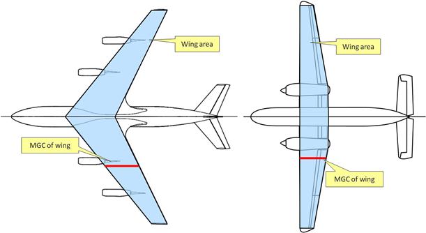
FIGURE 9-1 Reference area for the Boeing 707 and De Havilland of Canada DHC-7 Caribou (drawing is not to scale).
Since the definition of this area takes place in the early stages of the airplane’s design, it is almost always defined in a simple manner. As a consequence, when the geometry gets modified at a later time (for instance, a wingtip is reshaped) the reference area is not changed (as this would be likely to require a large number of documents to be revised, even certification documents), but the change will be manifested through a change in maximum lift coefficient, modified drag polar and similar definitions. An added wingtip shape, strakes, or leading edge extensions are typically omitted because they are often afterthoughts or added as a consequence of a wind tunnel or a flight test program (stall and spin recovery) or added features (wingtip tanks for greater range or modifications to the initial wing/fuselage fairing).
9.1.3 The Process of Wing Sizing
The concept of Wing Sizing refers to the process required to determine the size, shape, and three-dimensional positioning of the wing surfaces. This procedure is listed in Table 9-1.
TABLE 9-1
Initial Sizing and Layout Algorithm for the Wing of a GA Aircraft
| Step | Task | Section |
| 1 | It is assumed that the required wing area has already been determined using the constraint analysis method of Section 3.2, Constraint analysis. Verify the predicted stalling speed is within regulatory margins (e.g. 45 KCAS if LSA, 61 KCAS is 14 CFR Part 23, etc.) before proceeding. | 3.2 |
| 2 | Select the wing planform geometry (see Section 9.4, Planform selection). This may or may not be the final shape. | 9.4 |
| 3 | As a starting point, select a candidate aspect ratio and taper ratio. For AR consider the use of Equations (9-26) or (9-28). In the absence of specific target values, initial values can be selected by considering the class of aircraft being designed. For instance, refer to Tables 4-2 regarding the specific class of airplanes and then Tables 9-3 and 9-4 for additional help. These are initial values that are likely to change, but are a reasonable starting point. | 4.2 9.3.1 9.3.2 |
| 4 | Select candidate airfoils for the root and tip. Do not assign a wing washout at this time. | 8 |
| 5 | Evaluate the need for wing sweep. Is this a high-subsonic aircraft? Is there a possible problem with CG location that calls for a wing sweep to solve? | 9.3.3 |
| 6 | Once the airplane takes shape, a more sophisticated reshaping is required, in accordance with the design algorithm of Section 1.3.1, Conceptual design algorithm for a GA aircraft. This reshaping takes into account performance, stability and control, structural, and systems considerations. | 1.3.2 |
The Establishment of Basic Datum
The positioning of the wing is the determination of where, with respect to some reference point in space, the wing shall be located. During the design of the aircraft it is usually decided that the reference datum for the airplane may be a point on the fuselage or the wing or a point in space (typically ahead of the nose of the aircraft as discussed in Section 6.6.11, Center of gravity envelope).
Among those are evaluation of dynamic stability and compliance with the design checklist of Section 23.3, GA aircraft design checklist. Typically, this will consider the following:
• Stability derivatives such as Cmα, Cmδe, Cmq, Cyβ, Cnβ, Cnδr, Cnr, and others.
• Impact on the non-linear behavior of the above stability derivatives.
• Structures (structural weight, aeroelasticity, etc.).
• Control authority in extreme flight conditions.
• Operation (e.g. tail length may interfere with T-O rotation, require excessive control surface deflection, and subject the structure to high stresses, etc.).
• Stall tailoring; i.e. the design of the wing for benign stall characteristics.
9.2 The Trapezoidal Wing Planform
The trapezoidal planform represents the simplest geometric shape selected for aircraft lifting surfaces. Although basic, it is important enough to warrant a specific discussion. One of the primary advantages of this geometry is the simple mathematics that can be used to describe it. Absence of curvature or leading and trailing edge discontinuities results in a simple mathematical representation, in turn, offering convenience when sizing the airplane and extremely helpful when performing trade studies or during optimization.
This class of planform shapes includes a range of geometric shapes ranging from elementary forms, such as the constant-chord planform (“Hershey-bar”) to tapered planform shapes that may be swept forward or aft. It is important to know well the geometric relationships between span, aspect ratio, taper ratio, and chord. These will come in handy in a multitude of analyses, ranging from weight estimation to multi-disciplinary optimization.
Methods to treat planform shapes that are either cranked or described with piecewise continuous mathematical functions are given in Appendix D: Geometry of lifting surfaces.
9.2.1 Definitions
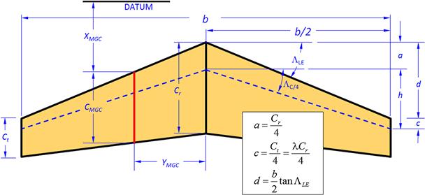
Figure 9-2 shows the general definitions for the geometry of the trapezoidal planform and indicates important details of such sections. A leading edge is the part of a lifting surface that faces the direction of intended movement. The trailing edge is opposite to that side. The root is the inboard side of the planform and, as can be seen in the figure, is where the two trapezoids join. This would typically be the centerline of the aircraft or the plane of symmetry. Although the term root sometimes refers to where the wing intersects the fuselage, that definition is not used in this text because the geometry of the fuselage may be changing and thus defining a wing chord there would lead to some undesirable issues. The tip is the side opposite of the root – it is the outboard side. The distance between the left and right tip is called the span, denoted by the variable b. The transverse dimension is called chord. Thus we talk about a root-chord or tip-chord as the length of the corresponding sides, denoted by the variables Cr and Ct, respectively. We also call the ratio of the tip-chord to the root-chord the taper ratio, denoted by λ. Another important ratio is the aspect ratio, AR, which indicates the slenderness of the wing. Both are expressed mathematically below.
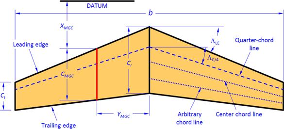
The quarter-chord line is drawn from a point one-fourth of the distance from the leading edge of the root-chord to a point one-fourth of the distance from the leading edge of the tip chord. It is important because two-dimensional aerodynamic data frequently uses the quarter-chord point as a reference when presenting pitching moment data. Scientific literature, for instance the USAF DATCOM, regularly uses the quarter-chord as a reference point for its graphs and computational techniques. Additionally, this is often the location of the main spar in lifting surfaces and it is very convenient to the structural analysts to not have to perform moment transformation during the design of the structure.
The center chord line is obtained in a similar fashion to the quarter-chord line and is sometimes used as a reference in scientific literature, although not as frequently. Other important parameters are the sweep angles of the leading edge and quarter-chord line, denoted by ΛLE and ΛC/4, respectively.
The mean geometric chord (MGC) of the planform is often (and erroneously) referred to as the mean aerodynamic chord (MAC), which is the chord at the location on the planform at which the center of pressure is presumed to act. The problem is that this location is dependent on three-dimensional influences, such as that of the airfoils, twist, sweep and other factors, not to mention angle-of-attack, in particular when flow separation begins. Authors who refer to the MGC as the MAC typically acknowledge the shortcoming, present the geometric formulation presented here to calculate it, before continuing to call it the MAC. In this text, we will break from this convention and simply call it by its appropriate title – the MGC. The importance of the MGC is that it can be considered a reference location on a wing, to which the location of the center of gravity is referenced and even for a quick preliminary estimation of wing bending moments inside it. Therefore, it is important to also estimate what its spanwise station, yMGC, is.
Considering Figure 9-2, we will now derive mathematical expressions for the aforementioned important properties of the wing:
![]() (9-1)
(9-1)
![]() (9-2)
(9-2)
Aspect ratio – constant-chord:
![]() (9-3)
(9-3)
![]() (9-4)
(9-4)
![]() (9-5)
(9-5)
![]() (9-6)
(9-6)
![]() (9-7)
(9-7)
![]() (9-8)
(9-8)
![]() (9-9)
(9-9)
![]() (9-10)
(9-10)
Angle of an arbitrary chord line:
![]() (9-11)
(9-11)
Equation (9-11) is obtained from USAF DATCOM [1], where m and n are chordwise fractions of the chord line (0.25 for quarter-chord, 0.5 for the center chord line, etc.) and m is the fraction for a known angle, and n for the unknown angle (see Example 9-1 for example of use).
Aspect Ratio for HT and VT
The aspect ratio for a horizontal tail (HT) is calculated exactly as it is for the wing. The aspect ratio for a vertical tail (VT) is calculated using the following expression:
The aspect ratio for a twin tail is calculated by applying Equation (9-12) to one tail only, where SVT refers to one half the total area of the VT.
Aspect Ratio for Multi-wing Configurations
The aspect ratio for multi-wing aircraft, such as biplanes and triplanes, is given below:
Derivation of Equations (9-6), (9-8), and (9-10)
Equation (9-6): see Section D.5.3, Derivation of MGC.
Equation (9-8): see Section D.5.2, Spanwise location of the MGC.
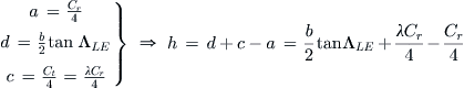
Equation (9-10): refer to the Figure 9-3 to define the dimensions a, b/2, c, d, and h.
![]()
![]()
EXAMPLE 9-1: TRAPEZOIDAL WING PLANFORM
Determine the primary characteristics of the wing shown in Figure 9-4. Also calculate the angle of the center chord line using Equation (9-11).

Solution
![]()
![]()
![]()
![]()
![]()
![]()
![]()
Angle of quarter-chord line:
![]()
Angle of the center chord line using the quarter-chord line (m = 0.25, n = 0.50) is obtained from Equation (9-11):
![]()
Inserting the given values, we get:
![]()
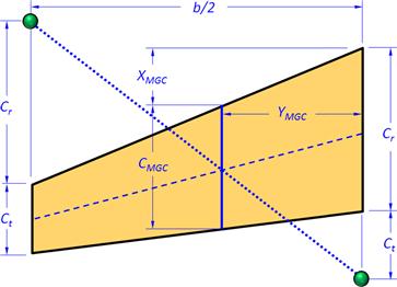
9.2.2 Poor Man’s Determination of the MGC
In the absence of computational tools the designer can determine the location of the MGC using the graphical scheme in Figure 9-5. It is important to remember that such graphical tools are the relics of a bygone era and at best are what the slide-rule is to the modern calculator – results from a digital calculator should always take precedence.
9.2.3 Planform Dimensions in Terms of S, λ, and AR
During the design phase, the basic dimensions of the wing (span and chord at root and tip) are sometimes defined by wing area, taper ratio, and aspect ratio as governing variables. This is convenient because these parameters can tell the designer a lot about the likely aerodynamic properties of the wing. With the wing parameters defined in this fashion use the following formulation to determine the required wingspan, root chord, and tip chord of a simple tapered planform like the one in Figure 9-6. These are based on Equations (9-2), (9-3), and (9-10):
Derivation of Equation (9-20)
Using Equation (9-18), we can calculate the root chord, Cr, using any set of values for the wingspan, b, and aspect ratio, AR:
![]()
We then insert this into Equation (9-6) and manipulate as follows:
![]()
QED
Derivation of Equation (9-21)
Parametric formulation of the chord c as a function of spanwise station y for a straight tapered wing whose taper ratio is λ, root chord Cr, and span is b is obtained by inserting the geometric parameters as follows (where the parameter t is 2y/b and ranges from 0 to 1):
![]()
QED
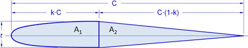
9.2.4 Approximation of an Airfoil Cross-sectional Area
Often, the cross-sectional area (internal area) of an airfoil must be evaluated as it yields useful clues about the internal volume of a wing available for fuel storage. In the absence of precise airfoil data the following approximation is used to estimate the internal area of geometry resembling that of an airfoil:
Sometimes it is more convenient to present the thickness using the thickness-to-chord ratio, denoted by (t/c). This way, the thickness is expressed using the product (t/c)·C. Thus, Equation (9-22) is written as follows:
Derivation of Equations (9-22) and (9-23)
Consider Figure 9-7, which shows an airfoil of chord C approximated by a parabolic D-cell and a triangular section. It is assumed the two sections join at the chord station of maximum thickness, t, whose location is given by k·C, where k is the location of the airfoil’s maximum thickness as a fraction of C. The cross-sectional areas of the two sections and the total area are given by the following expressions:
Therefore, the internal area of the airfoil can be approximated by adding the two as shown below:
![]()
Then, multiply by C/C (=1) to get Equation (9-23).
QED
9.3 The Geometric Layout of the Wing
Once the wing area and wingspan have been determined, it is possible to begin to establish the remaining geometric properties. The geometric layout of the wing refers to properties such as the aspect ratio, taper ratio, wing sweep, dihedral, and so on. These constitute the geometric layout of the wing. The layout has profound influence on the entire design process, affecting a large number of other areas in the development. These are not just aerodynamics, performance, and stability and control, but also structures and systems layout, just to name a few. The layout process assesses the topics listed below. The corresponding sections are listed as well.
The layout constitutes the geometric parameters presented in Table 9-2.
TABLE 9-2
Typical Values of AR for Various Classes of Aircraft
| Geometric property | Section |
| Planform shape | 9.4 |
| Aspect ratio (AR) | 9.3.1 |
| Taper ratio (TR or λ) | 9.3.2 |
| Leading edge (LE) or quarter chord (C/4) sweep angle | 9.3.3 |
| Dihedral angle | 9.3.4 |
| Washout | 9.3.5 |
| Angle-of-incidence | 9.3.6 |
| Positioning of the wing on the fuselage | 4.2.1 |
| Partitioning of the wing into a roll control region (ailerons), high lift region (flaps, slats), and lift suppression region (spoilers) | 10 |
Of these, the AR, TR, and the LE sweep give the designer fundamental control over the aerodynamic characteristics of the wing. This is not to say the others are not important too, but rather that they can be considered more as dials to “fine-tune” the wing design. The determination of the AR, TR, and sweep may be the consequence of a complicated optimization; however, this is not always the case.
9.3.1 Wing Aspect Ratio, AR
The wing aspect ratio (AR) is a fundamental property that simultaneously affects the magnitude of the lift-induced drag (CDi) and the slope of the lift curve (CLα). As such, it also directly influences both performance and stability and control. Table 9-3 shows typical values of the AR for several classes of aircraft.
TABLE 9-3
Typical Values of AR for Various Classes of Aircraft
| Type of Vehicle or Vehicle Component | AR Range |
| Missiles | 0.5–1 |
| Military fighters | 2.5–4.0 |
| GA aircraft | 6–11 |
| Aerobatic airplanes | 5–6 |
| Twin-engine commuters | 10–14 |
| Commercial jetliners | 7–10 |
| Sailplanes | 10–51 |
Figure 9-8 shows two planform shapes of equal planform area, but different AR. The stubby configuration (AR = 4) has a shallower CLα and lower CLmax, but higher stall AOA (αstall) than the slender one (AR = 16). The stubby planform has less roll damping than the high AR and, for that reason, is better suited for airplanes that require roll responsiveness, such as aerobatic aircraft. Additionally, it generates higher lift-induced drag (CDi) than the slender one. A high AR wing is required for sailplanes and airplanes that are required to have long-range or endurance. They have high roll damping and will be structurally heavier because of larger bending moments.
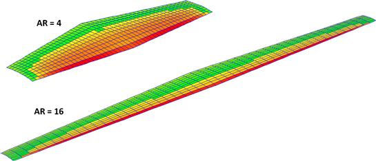
Table 9-4 gives a general rule-of-thumb about the impact the AR has on selected aerodynamic properties.
TABLE 9-4
Typical Impact of Aspect Ratio on Aerodynamic Properties of the Wing
| Aspect Ratio, AR | Pros | Cons |
| 1.0 | High stall angle-of-attack. High flutter speed. Low roll damping. Low structural weight. Great gust penetration capability (because of the shallow CLα). |
Inefficient because of high induced drag. Shallow CLα requires large changes in AOA with airspeed. Low CLmax (high stalling speed). Low LDmax. |
| 5–7 | Good roll response. Relatively high flutter speed. Limited adverse yaw. Reasonable gust penetration. |
Inefficient to marginally efficient for long-range design. Relatively high induced drag. |
| 7–12 | Good balance between low induced drag and roll response. Good glide characteristics for powered aircraft. |
Some adverse yaw may be noticed toward the higher extreme of AR. Resonable to marginal gust penetration capability (steep CLα). |
| 20+ | Low induced drag. Great glide characteristics. Steep CLα (large change in lift with small changes in α). High maximum lift coefficient. |
High structural weight. Low flutter speed. High roll damping. High adverse yaw. Steep CLα results in higher gust loads. |
The aspect ratio is defined as follows for monoplane and biplane configurations:
Illustrating the Difference Between Low and High AR Wings
The difference between a low and high AR is illustrated in Figure 9-9, which shows two wings of equal wing areas and taper ratios. The upper wing has a relatively low AR (6.67) while the lower one has a relatively large one (18.57). The airspeed in both cases is 100 KTAS and both are positioned at an AOA such they generate 2000 lbf of lift. The figure shows that the low AR wing requires an AOA of 1.55° but the high AR one 0.66°. In accordance with Section 15.3.4, The lift-induced drag coefficient: CDi, the higher AOA means the low AR wing generates higher induced drag. The greater flow field disruption is even visible by the larger wingtip vortex generated by the low AR wing in Figure 9-9. Here, a lift-induced drag value of 71 lbf was estimated for the low AR wing and 45 lbf for the high AR one. Additionally, the lift curve slope, CLα, for the low AR wing (4.475 per radian) is less than that of the high AR wing (5.459 per radian). Therefore, the low AR wing will stall at a higher AOA and airspeed than the high AR wing. However, it is far more responsive as its roll damping coefficient, Clp, is lower.
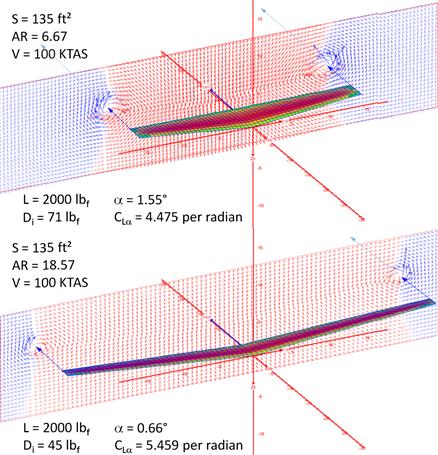
FIGURE 9-9 The difference between a low AR (top) and high AR (bottom) is illustrated. Both wings are of equal area and each generates 2000 lbf of lift at 100 KTAS. The flow solution is shown in a plane positioned aft of the wing trailing edge.
The difference between the two configurations is further illustrated in Figure 9-10. The graphs were generated for three wings using the potential flow theory. The wings all have a constant TR (0.5), but varying AR. The left graph shows the spanwise distribution of section lift coefficients at an AOA of 10°. The tip loading that results from the TR (and will be discussed next) is evident. It can be seen that the high AR of 16 generates the highest Cl at the give AOA, as is to be expected since its Clα is the highest. Other than the magnitude of the section lift coefficients, it is also evident that the AR does not have major changes on the general shape of the distribution; in other words, the AR has great effects on the magnitude of section lift coefficients at a given AOA, and relatively small influence on the shape of the distribution.
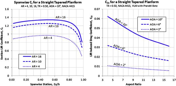
FIGURE 9-10 The left graph shows the spanwise distribution of section lift coefficients for three different ARs, while the right graph shows the effect of AR on the lift induced drag coefficient.
The left graph in Figure 9-10 shows how the AR affects the lift induced drag. This is illustrated for three AOAs; 2°, 6°, and 10°. The graph shows substantial reduction in lift-induced drag is to be had with larger AR.
Determining AR Based on a Desired Range
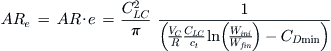
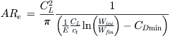
It is possible to evaluate and recommend AR for some special design cases. One such is the determination of AR based on a desired range, R, at some desired cruising airspeed, VC. If the aircraft being designed belongs to a class of aircraft for which CDmin can be estimated with reasonable accuracy and the expected initial and final cruise weights are known, denoted by Wini and Wfin, respectively, then the average cruise lift coefficient can be used with Equation (20-12) to extract the effective aspect ratio, ARe, for the vehicle using the following expression:
 (9-26)
where
CLC = average cruise lift coefficient, corresponding to the average of Wini and Wfin.
The denominator in Equation (9-26) results in a singularity when ![]() . In fact, it returns negative values if the airspeed is lower than obtained by the following expression:
. In fact, it returns negative values if the airspeed is lower than obtained by the following expression:
![]() (9-27)
(9-27)
For this reason, Equation (9-26) should only be applied to airspeeds that are greater than the value obtained by the above expression. It should be used to guide the selection of the AR rather than obtain it directly, for instance by plotting isobars.
Note that ARe is the product of the AR and Oswald’s span efficiency, AR·e. Once this product has been determined, it is the responsibility of the designer to devise a proper combination of AR and planform geometry to achieve this value. Also note that if the airplane features a swept back planform that the AR limits of Equation (9-94) must be considered as well.
Although the low AR surface is less efficient than the high AR, it is much better suited as a control surface for tail-aft configurations (i.e. as a horizontal and vertical tail). This results from the higher stall AOA, which is a consequence of the low AR. Delayed stall introduces a certain level of safety to the operation of tail-aft airplanes because it will require them to reach very high AOA or AOY before the stabilizing moments begin to drop. This is the reason why the horizontal and vertical tail surfaces on airplanes typically feature low aspect ratios.
Derivation of Equation (9-26)
Assuming the simplified drag model, Equation (20-12) can be solved for the drag coefficient as follows:
![]()
This can then be solved for the effective AR as follows:

Note that this is a generic case and the subscript C is used to denote some desired cruise conditions.
QED
EXAMPLE 9-3
The Cirrus SR22 pilot operating handbook (POH) reveals that the airplane has an 899 nm range at 65% power at 10,000 ft. The POH states the cruising speed at this condition is 174 KTAS and fuel consumption is 15.4 gal/hr. This implies an SFC = 15.4 gal/hr × (6 lbf/gal)/(0.65 × 310 BHP) = 0.4586 lbf/hr/BHP. Evaluate the reliability of Equation (9-26) by considering the hypothetical design of a SR22 class aircraft, which “happens” to share a number of parameters. This hypothetical airplane is designed for a range of 900 nm precisely at the same condition. Estimate the effective AR for this airplane using Equation (9-26) and compare to that of the SR22. Assume the weight at the beginning of cruise is 3379 lbf and 2910 lbf at end of cruise. Assume the wing area is 145 ft2 and CDmin = 0.02541 (as calculated per Example 15-18).
Solution
![]()
![]()
The airspeed in ft/s is 174 × 1.688 = 293.7 ft/s, so the lift coefficient at cruise is:
![]()
The thrust specific fuel consumption is found using Equation (20-9):
![]()
The desired range of 900 nm amounts to 5,468,400 ft, yielding the following effective AR:
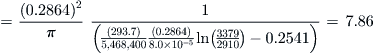
Note that the actual AR of the SR22 is 10. The answer therefore implies its Oswald efficiency is 0.786. This compares favorably to Equation (9-89) as follows:
![]()
Determining AR Based on Desired Endurance
The AR can also be determined based on a desired endurance, E, at some desired cruising airspeed, VC, similar to what was done for range and using the same basic variables. This time the method uses Equation (20-22) to extract the effective aspect ratio, ARe, for the vehicle using the following expression:
 (9-28)
where E = endurance in seconds.
Like Equation (9-26), the denominator in Equation (9-28) has similar limitations and should be used with cruise lift coefficients greater than those obtained with the following expression:
![]() (9-29)
(9-29)
Derivation of Equation (9-28)
Assuming the simplified drag model, Equation (20-22) can be solved for the drag coefficient as follows:
![]()
Note that this is a generic case and the subscript C is used to denote some desired cruise conditions.
QED
EXAMPLE 9-4
Use Equation (9-28) to estimate the effective AR for the SR22 class aircraft of Example 9-3, using the same parameters, if it is designed to cruise 900 nm at 174 KTAS.
Solution
Using Equation (9-28), the desired range of 900 nm at 174 KTAS amounts to 5.172 hrs, yielding the following effective AR:

effectively the same result as in the previous example.
Figure 9-11 shows the effect aspect ratio has on a wing’s lift curve and drag polar. It compares the properties of some airfoil (for which AR1 is considered ∞) to the same airfoil being used in a three-dimensional wing (whose AR2 is much, much smaller). It can be seen that as the AR reduces, so does the lift curve slope (denoted by Clα for the airfoil and CLα for the wing) and maximum lift coefficient (denoted by Clmax for the airfoil and CLmax for the wing). If the airfoil generates a specific lift coefficient at α1, it must be placed at a higher AOA, α2, once used on a three-dimensional wing. The cost of this is an increase in drag, which changes from Cd for the airfoil to CD for the wing, as is shown in Figure 9-11. The difference between the two is the three-dimensional lift induced drag coefficient and the rise in the airfoil drag due to growth in the flow separation region.

Estimating AR Based on Minimum Drag
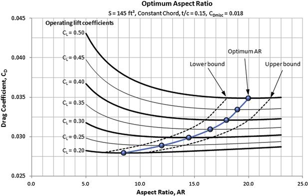
The AR can also be set based on the minimum drag of the airplane. This approach requires the design lift coefficient to be determined (e.g. see Equation [9-49]). Then, assuming constant wing area, a relatively sophisticated estimation of the total drag coefficient of the airplane is accomplished. The estimation takes into account changes in the wing geometry as a function of AR (wing chords change since S is constant) and evaluates skin friction assuming either a fully turbulent or a mixed boundary layer. Then, using the appropriate form and interference factors, the minimum drag coefficient is estimated (see Chapter 15, Aircraft drag analysis). The lift-induced drag coefficient is also calculated, using an appropriate model of the Oswald’s span efficiency. Adding the two coefficients comprises the total drag coefficient, CD. This can then be plotted versus the AR, in a carpet plot, similar to that of Figure 9-12. The carpet plot is usually prepared using a range of lift coefficients. Such a plot reveals the location of the optimum AR. The upper and lower bounds in the figure are simply the optimum AR ± 2, but the designer can widen or narrow this range depending on the project. Figure 9-12 shows that for the hypothetical aircraft being presented, practically any AR between the two limits will yield the lowest value of the total drag coefficient. This gives the designer room to accommodate other concerns such as structural weight.
Estimating AR for Sailplane Class Aircraft
A plausible AR for powered and unpowered sailplanes can be established using the historical data in Figure 9-13. The data points represent contemporary manufacturers’ information collected from Ref. [2]. The maximum lift-to-drag ratios (LDmax) presented includes the drag of the fuselage and stabilizing surfaces and demonstrates the sophistication of the modern sailplane. The graph shows trends for both regular and powered sailplanes and presents accompanying least-squares curves. Note that these estimates do not replace analyses of the kind presented by Ref. [3], but rather supply initial estimates based on historical sailplanes.
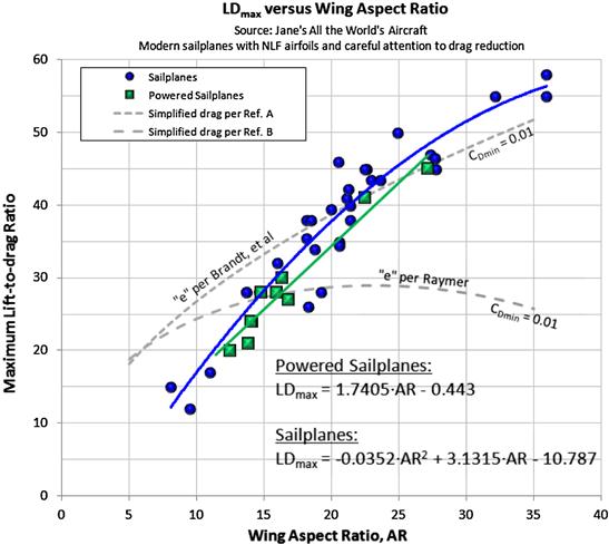
FIGURE 9-13 Maximum lift-to-drag ratio for modern sailplanes and powered sailplanes as a function of AR. Ref. A is Ref. [4] and Ref. B is Ref. [5].
Also plotted are theoretical predictions of the LDmax using the simplified drag model (see Chapter 15, Aircraft drag analysis) and CDmin of 0.01 (typical of many sailplanes). This model is often the first choice of the novice airplane designer, but it is inaccurate for sailplanes designed for extensive NLF as it does not model the drag bucket associated with such aircraft. These curves are merely presented here to demonstrate why the simplified drag model is a poor predictor.
The theoretical LDmax was calculated using Equation (19-18), where the Oswald’s span efficiency was calculated per Equations (9-91) and (9-89) and. The curves shown assume a minimum drag coefficient of 0.01, which is a typical value for clean sailplanes. The graph shows clearly the limitation of the simplified drag model.
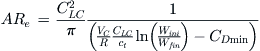
The following empirical formulation can be used to estimate the AR for the conceptual design of unpowered and powered sailplanes (as long as AR < 36):
Naturally, the calculated AR will not guarantee that a desired LDmax will be achieved. Rather it indicates that, historically, sailplanes with that AR have achieved the said LDmax. Achieving it will require the utmost attention to anything on the airplane that generates drag.
9.3.2 Wing Taper Ratio, TR or λ
The taper ratio is the second of the three most important geometric properties of a wing. It has a profound impact on how lift is distributed along the wingspan. For instance, consider Figure 9-14, which shows how it changes the spanwise distribution of section lift coefficients (left graph) and lift force per unit length (right graph). It shows clearly how a highly tapered wing becomes “tip-loaded,” whereas a constant-chord wing is “root-loaded,” terms that refers to the distribution of section lift coefficients. This is of great importance when tailoring stall characteristics and controlling the effectiveness of the wing. The right graph shows how the actual lift force of the highly tapered wing moves inboard. This reduces the bending moments and can help reduce the structural weight of the wing.

FIGURE 9-14 The effect of taper ratio on the spanwise distribution of section lift coefficients (left); and lift force (right).
Too much tip-loading of a wing can have serious consequences for its stall characteristics. It is evident from the shape of the spanwise Cl that the wing whose TR = 0.2 will stall near the wingtip, as it peaks there. This would make the wing very susceptible to roll instability at stall, which could have dire consequences if ignored. The constant-chord wing, on the other hand, has its Cl peak inboard, near the root, which retains roll stability and results in benign stall characteristics. Such characteristics are very desirable for trainers and, frankly, should be one of the primary goals of any passenger-carrying aircraft.
Additionally, the left graph of Figure 9-14 shows that a TR in the neighborhood of 0.5–0.6 is a good compromise between efficiency and stall behavior, even though some wing twist (to be discussed later) will be required to ensure stall progression that protects roll stability at stall. The right graph of Figure 9-14 shows that even though the outboard airfoils of the highly tapered wing are working hard to generate lift, the actual force is less than that of the constant-chord wing because the chord is so much shorter. This is very beneficial from a structural standpoint as it brings the center of force inboard and reduces the wing bending moments, although torsional rigidity on the outboard wing suffers. Table 9-5 gives a general rule-of-thumb about the impact the TR has on selected aerodynamic properties.
TABLE 9-5
Typical Impact of Taper Ratio on Aerodynamic Properties of the Wing
| Taper Ratio, λ | Pros | Cons |
| 0.3 | Induced drag is close to that of an elliptical wing planform, but is much simpler to manufacture. | Poor stall characteristics. Tip-loaded planform requires a large washout to delay tip stall. |
| 0.5 | Good balance between low induced drag and good stall characteristics. | Stall begins mid-span and spreads to tip and root. Usually requires moderate washout. |
| 1.0 | Good stall progression. Washout generally not required. Simple to manufacture. | High induced drag. |
9.3.3 Leading Edge and Quarter-chord Sweep Angles, ΛLE and ΛC/4
The purpose of sweeping the wing forward or aft is primarily twofold: (1) to fix a CG problem and (2) to delay the onset of shockwaves. The latter is the reason for using swept wings for high-speed aircraft (high subsonic and supersonic). However, the former is surprisingly common as well. Strictly speaking, sweep should be avoided unless necessary. It not only makes the wing less efficient aerodynamically, it is also detrimental to stall characteristics if swept back. Additionally, for slow-flying GA aircraft, it implies the spar has discontinuous breaks in it that make it less efficient structurally.
Of course, this is not to say that sweep is all bad. It is very helpful for the design of high-speed aircraft, where it enables the use of thicker airfoils, which lightens the airframe and makes up for some of the lost efficiency. For low-speed airplanes, it is a tool that allows a project to be salvaged if it is discovered that the CG is farther forward or aft than anticipated. This is the reason behind the aft-swept wings featured on the venerable Douglas DC-3 Dakota (C-47) [6]. The same holds for forward-swept configurations. The military scouting and trainer airplane SAAB MFI-15 Safari was designed with an improved field-of-view in mind, which is why it features a shoulder-mounted wing with the main spar behind the two occupants. The wing is swept forward to solve the CG issue that results from the engine and the two occupants sitting in front of the main spar.
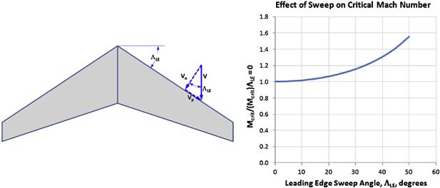
Impact of Sweep Angle on the Critical Mach Number
The greatest benefit of wing sweep is a reduction in the strength of and delay in the onset of shock formation. The shock formation will not only cause a sharp increase in drag; it also changes the chordwise pressure distribution on the airfoil, causing the center of lift to move from approximately the airfoil’s quarter-chord to mid-chord. The consequence of this is called “Mach-tuck,” a severe increase in nose-down pitching moment. The change in drag due to this effect is detailed in Section 15.4.2, The effect of Mach number. Also, Figure 15-28 shows how the leading edge sweep increases the critical Mach number, Mcrit, and delays the onset of the peak of the compressibility drag coefficient. This is helpful as it allows thicker and more structurally efficient airfoils to be used in the wing.
Consider the swept wing in Figure 9-15 and the deconstruction of the far-field airspeed into two components: one parallel to and the other perpendicular to the leading edge. In its simplest form the wing sweep theory contends that it is the airspeed component normal to the leading edge that dictates when shockwaves begin to form. This allows the following correction to the critical Mach number to be made (see Section 8.3.7, The critical Mach number, Mcrit).
![]() (9-32)
(9-32)
In practice, only half of this reduction is experienced.
Impact of Sweep Angle on the CLmax
The maximum lift coefficient is reduced with an increase in wing sweep angle. This is detailed in Section 9.5.10, Step-by-step: Rapid CLmax estimation.
Impact of Sweep Angle on Structural Loads
The sweep has very important effect on structural loads. As discussed in Chapter 8, The anatomy of the airfoil, cambered airfoils inherently generate a pitching moment about their quarter chords whose tendency is to rotate the airfoil LE down. All flapped airfoils, cambered or not, generate extra pitching moment (torsion), which is added to the baseline moment. The total moment, regardless of composition, is reacted as shear flow in the wing structure. If the wing is swept aft, an additional and usually much larger pitching moment is generated because of the center of lift being moved a large distance aft. Consequently, the swept wing structure will be heavier than a straight wing designed for the same flight condition. Similarly, a forward-swept wing may also introduce a large LE up torsion, if the sweep angle is large enough, although this is reduced by an amount corresponding to the innate torsion of the airfoils of the wing.
Impact of Sweep Angle on Stall Characteristics
Sweep angle has very detrimental effects on the stall characteristics for reasons detailed in Sections 9.6.5, Cause of spanwise flow for a swept-back wing planform and 9.6.6, Pitch-up stall boundary for a swept-back wing planform.
9.3.4 Dihedral or Anhedral, Γ
The dihedral (or anhedral) is the angle the wing makes with respect to the ground plane or the x-y plane (as it is normally called) when viewing the airplane from the front (or back). A dihedral refers to the wingtip being higher (with respect to the ground) than the wing root. The opposite holds true for anhedral. The dihedral affects the lift of the configurations in two ways: due to the tilting of the lift force and how the dihedral changes the AOA of the wing. Consider a wing that has dihedral angle Γ subjected to an AOA given by α. The geometry of the configuration reveals that the AOA seen by the airfoil, and denoted by αN, is reduced by the factor cos Γ (for instance, if Γ = 0°, then αN = α and if Γ = 90°, then αN = 0°, no matter the magnitude of α). Therefore, we can write:
![]() (9-33)
(9-33)
Similarly, the lift generated in the plane of symmetry is the product of the lift normal to the wing surface, denoted by LN, reduced by the same factor, cos Γ.
![]() (9-34)
(9-34)
Since LN can be written as ![]() , the lift in the plane of symmetry can be presented as follows:
, the lift in the plane of symmetry can be presented as follows:
![]() (9-35)
(9-35)
where
This result has been experimentally confirmed, for instance see Ref. [7]. It allows wing lift to be determined in terms of variables that refer to a wing with no dihedral. Furthermore, see discussion of V-tails in Section 11.3.4, V-tail or butterfly tail. Typical wings feature a dihedral of 4°–7°. The term cos2 Γ amounts to 0.995 to 0.985 and, therefore, is usually ignored in the estimation of stability derivatives.
Dihedral plays an essential role in the generation of dihedral effect. It is discussed further in Section 4.2.3, Wing dihedral. Values for several classes of aircraft are given in Table 9-6.

9.3.5 Wing Twist – Washout and Washin, ϕ
Many aircraft feature wings that are twisted so the tip airfoil is at a different angle of incidence with respect to the fuselage than the root airfoil. This is called wing washout if the incidence of the tip is less than that of the root, and washin if it is larger. Washin is rarely used, but is mostly used to describe the aeroelastic effects high AOA has on forward-swept wings, where aerodynamic loads tend to twist the wing so the AOA at the tip is increased even further. This article, however, deals with the intentional twisting of the wing, where its purpose is generally twofold:
1. To prevent the wingtip region from stalling before the wing root. If the wingtip stalls before the root, there is an increased risk the aircraft will roll abruptly and uncontrollably at stall, a condition that may lead to incipient stall. Roll tendency at stall contributes significantly to fatal accidents1 as it will often take place at low altitudes when an airplane banks to establish final approach before landing. An aircraft with such a roll-off tendency may stall if the pilot banks steeply and it may, ultimately, result in a crash as lack of altitude will prevent successful recovery. In the real world, manufacturing tolerances inevitably lead to airplanes not being perfectly symmetrical. This promotes one side of the airplane to stall before the other one, generating a rolling moment at stall. A wing twist can be used to build a “buffer” so the wingtips remain un-stalled when the rest of the wing stalls, greatly improving roll stability.
2. To modify the spanwise lift distribution to help achieve minimum drag at mission condition. The wing is most efficient when the section lift coefficients are constant along the span, as it is for an elliptical wing planform. Twisting the wing will allow the spanwise distribution of section lift coefficients to be modified for a tip-loaded wing, bringing the general distribution closer to that of an elliptical wing. A byproduct of this is a reduction in wing bending moments as the center of lift is brought closer to the plane of symmetry.
Geometric Washout
Geometric washout usually refers to the difference in angles of incidence of the root and tip airfoils (see Figure 9-16). It is denoted by ϕG. Generally the wing twist ranges from 0° to −4°, where the negative sign indicates that the leading edge of the tip is lower than that of the root. Thus, if we say the “washout is 3°” we mean that ϕG = −3° and the LE of the tip is lower than that of the root. If we say the “washin is 3°” we mean that ϕG = +3° and the LE of the tip is higher than that of the root. For instance, the inserted image of the root and tip airfoils in Figure 9-16 displays a washout. However, sometimes twist is highly complicated along the wingspan as in the case of the McDonnell-Douglas AV-8B, whose twist varies in a segmented fashion to a maximum of −8° at the tip [8].

Note that if the twist is linear, the relative angle of twist at any spanwise station can be determined using the following expression:
![]() (9-36)
(9-36)
The expression assumes the reference angle is 0 when y = 0 (the plane of symmetry) and becomes ϕG at the wingtip (where y = b/2).
Aerodynamic Washout
Aerodynamic washout is another way of designing roll stability at stall into the wing. In this case, two different airfoils are selected for the root and tip that are specifically based on one of two parameters: (1) their individual zero-lift AOA or (2) their two-dimensional stall AOA or maximum section lift coefficient. The former is favored when analyzing wings using methods such as the lifting line theory. Typically the idea is to provide roll stability at high AOA by ensuring the tip airfoil remains un-stalled before the inboard airfoil.
The primary reason for selecting an aerodynamic washout is that it allows the main wing spar caps to be straight, something that is important for the construction of composite aircraft. A spar cap in a composite aircraft mostly consists of unidirectional fibers, whose strength is very sensitive to fiber alignment. Once two airfoils have been selected, the aerodynamic washout is defined as follows (see Figure 9-17):
![]() (9-37)
(9-37)
![]() (9-38)
(9-38)
where
![]() = two-dimensional zero-lift AOA for the root airfoil
= two-dimensional zero-lift AOA for the root airfoil
![]() = two-dimensional zero-lift AOA for the tip airfoil
= two-dimensional zero-lift AOA for the tip airfoil
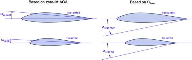
Note that there is an inherent problem with the definition based on Equation (9-37) and this is displayed in Figure 9-18. To begin with, the left graph of Figure 9-18 depicts the idea behind the aerodynamic washout: that the root airfoil stalls at an AOA less than the tip. It assumes that (1) αZL tip – αZL root = αstall root – αstall tip, which is not necessarily achieved in practice, and (2) requires CLmax tip = CLmax root (otherwise assumption (1) will not hold). This allows the aerodynamic washout can effectively be represented as the difference in the zero-lift AOAs.
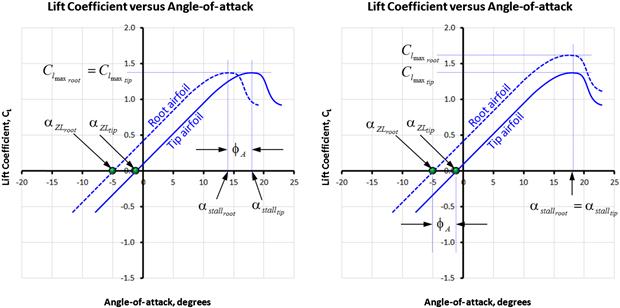
FIGURE 9-18 Idealized effect of an aerodynamic washout. In the left graph, the root airfoil stalls at a lower AOA than the tip providing roll stability at stall. A problem for the zero-lift definition of the aerodynamic washout is shown to the right. The root airfoil has a higher Clmax than the tip airfoil but stalls at the same AOA; the effective washout is zero. This renders the definition of washout based on zero-lift angles misleading.
One of the problems with this definition is shown in the right graph of Figure 9-18, which depicts the common case of the root airfoil being thicker than the tip airfoil. Consequently, its Clmax may be larger than that of the tip airfoil and its stall AOA is greater. Furthermore, if the wing is tapered, the difference in Reynolds number between the two can make the CLmax tip and αstall tip substantially smaller than that of the root. The figure effectively depicts a scenario in which the true washout is zero and possibly a washin, whereas relying on the zero-lift AOAs might indicate ample washout and therefore is misleading. Additional complexity must be considered in the magnitude of the section lift coefficients, which vary along the span. The above definition, thus, only gives a part of the whole picture; the remainder calls for analysis of the distribution of section lift coefficients along the span.
A Combined Geometric and Aerodynamic Washout
If two different airfoils are selected for the root and tip, in addition to a geometric washout, the combined effect can be calculated from:
![]() (9-39)
(9-39)
EXAMPLE 9-5
An airplane features two dissimilar airfoils at the root and tip whose αstall root = 16.5° and αstall tip = 15.0°. What is the combined washout for a geometric washout of 0° and 3°?
Panknin and Culver Wing Twist Formulas
The wing twist of a flying wing is such a fundamental parameter that it should be determined early on in the design phase – effectively as soon as the design lift coefficient has been determined. The designer of tailless aircraft can determine the proper washout of the wing using one of two special formulas specifically devised to help with the layout of such configurations. They are called the Panknin and Culver twist formulas. They are presented here without derivation for completeness of the discussion in this article.
The Panknin twist formula is attributed to Dr. Walter Panknin, who in 1989 presented a method to the designers of radio-controlled (RC) aircraft intended to help them properly lay out the washout of flying wings so the elevons are in trail at cruise. The formulation has been applied with great success to many RC flying wing designs [2]. It determines the geometric twist ![]() between the inboard and outboard airfoils of the wing (see Figure 9-19) using the following expression:
between the inboard and outboard airfoils of the wing (see Figure 9-19) using the following expression:
![]() (9-40)
(9-40)
where
![]() = pitching moment coefficient of the tip airfoil
= pitching moment coefficient of the tip airfoil
![]() = pitching moment coefficient of the tip airfoil
= pitching moment coefficient of the tip airfoil
![]() = lift coefficient at cruise (for which the aircraft is designed)
= lift coefficient at cruise (for which the aircraft is designed)
KSM = fraction design static margin (e.g. if SM = 10% then KSM = 0.1)
![]() = zero-lift AOA for the root airfoil, in degrees
= zero-lift AOA for the root airfoil, in degrees
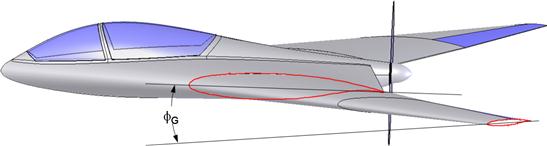
The formula determines the geometric twist angle ![]() based on the selected static margin, but allows the designer to select airfoils, AR, and quarter-chord sweep angle. It is applicable to both forward- and aft-swept wings. Note that one must exercise care in the application of units for the quarter-chord sweep. Its units must be in terms of degrees.
based on the selected static margin, but allows the designer to select airfoils, AR, and quarter-chord sweep angle. It is applicable to both forward- and aft-swept wings. Note that one must exercise care in the application of units for the quarter-chord sweep. Its units must be in terms of degrees.
The Culver twist formula is attributed to Mr. Irv Culver, a former engineer at Lockheed Skunk Works. Like the Panknin formula, his formula is widely used by designers of small RC tailless aircraft. It is intended for flying wings of moderate sweep angles (typically ≈20°) and design lift coefficients of 0.9–1.2, where the lower value indicates a high-speed glider and the higher is for high-performance sailplanes [8]. Note that the presentation here differs slightly from that of Ref. [8] in the simplification of terms.
![]() (9-41)
(9-41)
where
Once the washout is known its distribution along the span can be found using the following expression:
![]() (9-42)
(9-42)
EXAMPLE 9-6
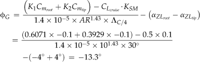
A flying wing is being designed for operation at a cruise CL of 0.5 (CLC = 0.5) at a static margin of 10% (KSM = 0.1). It has been determined that its AR shall be 10, taper ratio (λ) shall be 0.5, and quarter-chord sweep angle, ![]() , is 30°. During the airfoil selection process, the designers compare the use of a NACA 4415 airfoil (a conventional highly cambered airfoil, whose Cm is −0.1 and αZL = −4°) and a NACA 0015 airfoil (whose Cm is 0.0 and αZL = 0°). What is the required washout using each airfoil, in accordance with the Panknin formula?
, is 30°. During the airfoil selection process, the designers compare the use of a NACA 4415 airfoil (a conventional highly cambered airfoil, whose Cm is −0.1 and αZL = −4°) and a NACA 0015 airfoil (whose Cm is 0.0 and αZL = 0°). What is the required washout using each airfoil, in accordance with the Panknin formula?
Solution
The solution is effectively “plug and chug” into Equation (9-40). First, the parameters K1 and K2 must be determined.

Using these with Equation (9-40) for the NACA 4415 airfoil leads to:
Using these with Equation (9-40) for the NACA 0015 airfoil leads to:

The analysis shows that using a conventional cambered airfoil like the NACA 4415 is a bad choice, as it would require a 13.3° washout. Using a symmetrical airfoil like the NACA 0015 would bring this down to 4.42°.
9.3.6 Wing Angle-of-incidence, iW
Once the general shape of the fuselage, wing, and horizontal tail has been selected, it is time to decide on the relative orientation of the three. Consider a commercial jet designed to cruise at a specified airspeed, VC, and altitude (e.g. M = 0.8 at 35,000 ft). Once the desired cruise altitude has been reached, we note the weight of the airplane at the beginning of its cruise segment as W1. We also note its weight at the end of the cruise segment as W2. It should be evident that if the airplane is operated using conventional fossil fuel, then W1 will be greater than W2. This is particularly true for jet aircraft as large quantities of fuel are consumed en route. Consequently, the airplane will initially be cruising at a higher AOA than at the end of its mission. Keeping the change in AOA in mind it is prudent to determine the AOA at mid-cruise and use this as a representative AOA for the entire cruise segment. This AOA will be closer to both the initial and final AOAs than if either the initial or final AOA were selected.
Now consider Figure 9-20, which shows three possible orientations of a fuselage during the cruise. The top fuselage has its nose too low, the center too high, and the bottom one shows the correct orientation. Note that all three fuselage placements show a representative root airfoil mounted at the same cruise AOA (or αC) – it is only the fuselage that is mounted differently. Note that it is more convenient to refer the wing incidence to the root airfoil rather than the MGC airfoil, because this is usually directly referred to in the fuselage lofting.
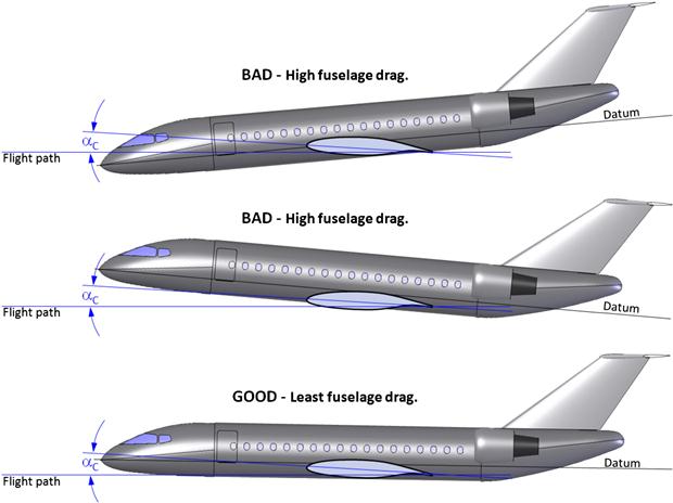
FIGURE 9-20 Determination of the fuselage minimum drag position. The two top configurations will generate greater drag at cruise than the bottom one, which places the fuselage in its minimum drag orientation at cruise. For a conventional pressurized aircraft the centerline of the fuselage will be close to parallel to the flight path during cruise.
The two top schematics in Figure 9-20 show fuselage and wing configurations that result in a higher total airplane drag than the bottom one. It is the responsibility of the designer to determine the optimum AOA for the fuselage and make sure this is the orientation of the fuselage at the selected cruise mission point. This AOA may be based on the minimum drag position of the fuselage, or its maximum lift-to-drag ratio, or its maximum lift contribution when combined with the wing. In other words, the optimum AOA of the fuselage should be determined as the one that maximizes the efficiency of the airplane as a whole. For instance, a minimum drag AOA for a typical commercial jetliner fuselage would be close to being parallel to the flight path during the design cruise condition and then the wing should be mounted at its required representative cruise AOA at that condition. The determination of the wing AOI can be considered a four-step process. The first step is to determine the fuselage minimum drag AOA, the second is to determine the required cruise AOA, the third is to add the two together, and the fourth is to determine the horizontal incidence angle that minimizes trim drag.
Step 1: Determine the Optimum AOA for the Fuselage
The first step will be highly dependent on the geometry of the aircraft, although when considering fuselages for conventional commercial aircraft it is good to assume it is parallel to the centerline of the tubular structure that forms the passenger cabin (see the datum in Figure 9-20). A wind tunnel testing or a CFD analysis should be used to determine the optimum orientation of the fuselage as its influence on the three-dimensional flow field may be quite complicated. The result from this step would be denoted by αFopt, for AOA of optimum fuselage orientation, using the following stipulation:
Step 2: Determine the Representative AOA at Cruise
The value of the midpoint cruise AOA, αC, can be determined from Equation (9-43) below:
![]() (9-43)
(9-43)
where
Step 3: Determine the Recommended Wing Angle-of-incidence
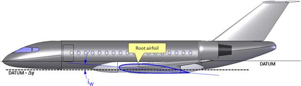
The angle-of-incidence (see Figure 9-21) at the root airfoil, denoted by iW, can now be determined from:
![]() (9-44)
(9-44)
where
Note that since the first two terms of the above expression really return the AOI at the MGC rather than at the root, a correction must be introduced if the wing features a washout. This is denoted by the term ΔϕMGC, which is the difference in angular incidences between the root and MGC airfoils. If the wing has a linear twist the value of ΔϕMGC can be determined as follows by inserting the expression for the spanwise location of the MGC, yMGC, of Equation (9-8) into Equation (9-36). Note that the minus sign in Equation (9-44) is required to ensure that a washout will be added to determine:
![]() (9-45)
(9-45)
Step 4: Determine the Recommended HT Angle-of-incidence
Once a recommended wing AOI has been determined, the incidence of the HT can be determined. Again using the representative cruise mission weight (W1 + W2)/2 the horizontal tail should be mounted so the elevator deflection at this point will be neutral. This is called flying the horizontal in trail and simply means neutral deflection. This will result in a minimum trim drag.
Derivation of Equation (9-43)
Assuming the general lift properties of the wing are known, the lift coefficient can be written as follows combining either Equation (9-43) or (9-50):
![]() (i)
(i)
The weight of the airplane at the midpoint during the cruise is the average of the initial cruise weight, W1, and the weight at the end of cruise, W2:
![]() (ii)
(ii)
Where αC is the midpoint cruise AOA. Solving for αC leads to:
![]()
The last term is simply the zero lift AOA, αZL, which can be seen from:
![]()
Derivation of Equation (9-45)
Assuming the general lift properties of the wing are known, the lift coefficient can either be written as follows combining Equations (9-43) or (9-50):
![]()
QED
EXAMPLE 9-7
A reconnaissance aircraft is being designed and is expected to weigh 20,000 lbf at the start of its design mission cruise segment at a cruising speed VC = 250 KTAS at 25,000 ft, and 15,500 lbf at the end. Determine a suitable angle-of-incidence for its wing if the following parameters have been determined (ignore compressibility effects):
where
CLα = lift curve slope = 4.2 per radian
b = reference wingspan = 52.9 ft
S = reference wing area = 350 ft2
αZL = zero lift angle-of-attack = −2.5°
Solution
Step 1: Establish the optimum AOA for the fuselage. Since the fuselage minimum drag position is 1.2° nose up, we set αFopt = −1.2°.
Step 2: Determine the representative AOA at the midpoint of the cruise segment (note that density at 25,000 ft is 0.001066 slugs/ft3).
![]()
In other words, the MGC should be approximately at an AOA of 4.8° at the midpoint of the cruise. On a completely different note, at an initial wing loading of 20,000 lbf/350 ft2 = 57.1 lbf/ft2, the designer may want to reconsider whether this airplane should have a greater wing area. Let us not digress.
Step 3: Determine the recommended AOI based on the minimum drag configuration of the fuselage at the cruise midpoint. First, calculate the correction angle since the wing has a 3° washout.
![]()
Then, finish by calculating the recommended AOI for the wing root chord as follows:
![]()
It can be seen that the AOA of the MGC is given by αC and is 4.789° and if the fuselage optimum AOA were 0°, rather than −1.2°, the recommended AOI would be 4.789° − (−1.333°) = 6.122°. The resulting geometry is shown in Figure 9-22.

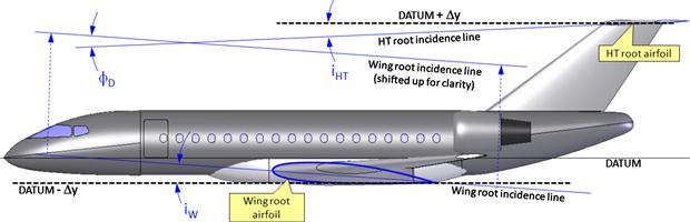
Decalage Angle for a Monoplane
On a monoplane, a decalage angle is the difference between the incidence angles of the wing and horizontal tail: Figure 9-23. The angle is an important indicator of the stability of the aircraft and generally requires substantial stability analyses to determine. Strictly speaking, the AOI of the HT, iHT, is determined based on the wing AOI, iW, and then the decalage angle can be calculated as shown below:
![]() (9-46)
(9-46)
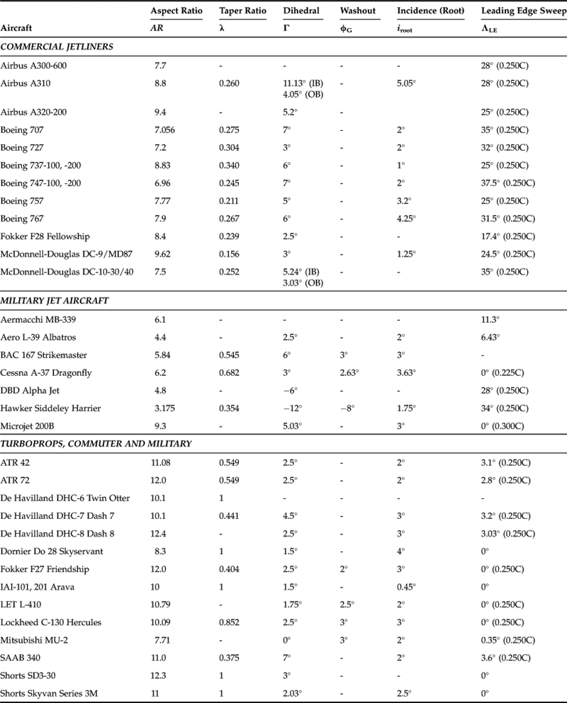
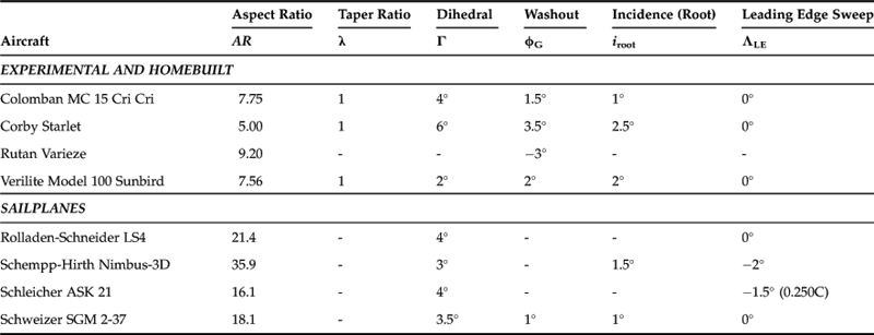
9.3.7 Wing Layout Properties of Selected Aircraft
The purpose of Table 9-6 is to present the reader with typical values of some of the wing parameters presented above to help assessing appropriate values.
9.4 Planform Selection
As stated in the introduction to this section, a glance at the history of aviation reveals a large number of planform shapes have been used. The success of some is glaring (e.g. constant-chord, tapered, swept back), while others have been a disappointment (e.g. triplanes, disc-shaped, circular, channel wings). This section evaluates the impact of varying the wing planform shape on the wing’s capability to generate lift and to lose it at stall.
For convenience, the distribution of the section lift coefficients for the planform shapes will be compared to that of a rectangular constant-chord wing. This is done to help the reader realize the impact of selecting a particular geometry. All the planform shapes feature the same reference area (10 ft2), the same airfoil (NACA 4416), and are exposed to airspeed of 100 KCAS at a 10° angle-of-attack. They should be thought of as a wing planform study for a generic airplane, so the physical geometry should be ignored and they should rather be evaluated in terms of parameters such as their aspect ratio (AR), taper ratio (TR), and leading edge sweep angles. Wing dihedral and washout is 0° for all examples. The AR and TR are varied to ensure all the examples have an equal area, while featuring values that are representative of typical airplanes. This gives an excellent insight into the lifting capabilities of the planform. Examples of aircraft that use the said planform shapes are cited as well. The reader should be aware that the true maximum lift coefficient of each wing planform shape will ultimately depend on the airfoil selection and various viscous phenomena. Such effects are too complicated to deal with in general terms in this text and may have a profound impact on the actual stall characteristics.
9.4.1 The Optimum Lift Distribution
Generally, the objective during planform selection is to select geometry that (1) generates lift through an effective use of the available span, (2) does not generate excessive bending moment, (3) results in docile stall characteristics, and (4) offers acceptable roll responsiveness. Let’s consider these in more detail.
Figure 9-24 shows the distribution of section lift coefficients, Cl, along the span of some arbitrary wing planform. The figure shows the frontal view of a cantilevered wing (the left wing is shown, looking toward the leading edge). The plane of symmetry (left) is where the wing root would be located and the right side is the left wingtip. The figure shows two kinds of distribution of Cl. The first can be considered an ideal spanwise distribution, which would be achieved if the laws of physics didn’t require the lift to gradually go to zero at the wingtip. This distribution would result in each spanwise station contributing uniformly to the total lift coefficient. As a consequence, it would require the least amount of AOA at any given airspeed to maintain altitude. And as is shown in Chapter 15, the less the AOA, the less is the generation of lift-induced drag.
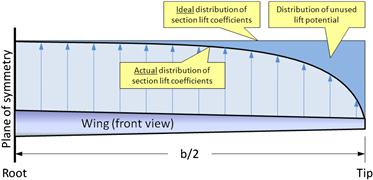
Figure 9-24 also shows the actual distribution of Cl. It represents the true section lift coefficients generated along the wing and it differs from the ideal distribution. Thus, the area between the ideal and actual distributions represents the distribution of unused lift potential. The smaller this area, the more efficient is the wing. The larger this area, the higher will be the stalling speed of the aircraft, because the missing lift must be made up for with dynamic pressure (i.e. airspeed) at stall. Similarly, the larger this area, the greater will be the induced drag at cruise, because the missing lift, again, must be made up by a larger AOA (which implies an increase in pressure and induced drag). In short, the design goal of the lifting surfaces should always be to minimize the wasted lift distribution.
Unfortunately, things are a bit more complicated than reflected by this. It turns out that wings designed to generate as uniform a distribution of Cls as possible have a serious side effect: stall. Theoretically, if such a wing uses an identical airfoil (ignoring the viscous effects), every spanwise station stalls at the same instant. In real airplanes this causes the wing to roll to one side or the other, depending on factors like yaw angle, propeller rotation, deviations from the ideal loft, and others. A wing roll-off at stall can initiate a spin – a very dangerous scenario if the airplane is close to the ground, such as when maneuvering (banking) to establish final approach before landing. For this reason, some of the efficiency must be sacrificed for added safety in the handling the airplane, using techniques such as wing washout, dissimilar airfoils, discontinuous leading edges, and many others.
It turns out that there actually is a wing planform that, at least in theory, achieves the ideal lift distribution; the elliptic planform (see Section 9.4.4, Elliptic planforms). The planform will generate section lift coefficients that are uniform along the entire span (see Figure 9-25). Unfortunately, as always, there is a catch – a very serious catch. The uniform distribution achieved by the elliptic planform is great for cruise, but awful near stall. As the elliptic planform reaches higher and higher AOA, the wing will stall fully – instantly, rather than progressing gradually from the inboard to the outboard wing, something that helps to maintain roll stability. This means that if there are manufacturing discrepancies – and there always are manufacturing discrepancies – the left or right wing may stall suddenly before the opposite wing. The consequence is a powerful wing roll to the left or right. This tendency can be remedied by a decisive wing washout; however, the resulting distribution of section lift coefficients will no longer be uniform. It is also possible to help stall progression with stall strips; however, whatever the remedy, the project will possibly be hampered by a troublesome stall improvement development during flight testing.
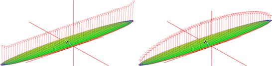
FIGURE 9-25 The difference between the distribution of section lift coefficients (left) and lift force (right). The distribution of section lift coefficients is indicative of stall tendency and induced drag coefficient. The lift force distribution is important for structural issues.
Another important observation can also be made from Figure 9-25. This is the difference between the distribution of section lift coefficients and that of lift force. While the distribution of section lift coefficients is a very important indicator of stall tendency and induced drag coefficient, the lift force distribution is imperative for structural reasons. The vertical shear force can be determined by integrating the distributed lift force along the span. Bending moments are obtained by integrating the shear along the span. With this in mind, the right graph of Figure 9-14 effectively shows how low taper ratio reduces the wing bending moments by moving the center of the lift inboard. For this reason tapered wings are essential to help reduce structural weight.
All the following images assume the leading edge faces up and the trailing edge down, and simple expressions of wing area and AR are provided for convenience. Always be mindful of the difference in Reynolds numbers for tapered wing planform shapes (root Re is different from tip Re). This comparison is implemented via the vortex-lattice method (VLM) using the commercially available code SURFACES [10]. All the models have 720 panels and are aligned along the camber line of the NACA 4416 airfoil.
9.4.2 Methods to Present Spanwise Lift Distribution
The lift distribution is usually presented in three forms: force distribution, section lift distribution, and a distribution of the fraction of section lift coefficients to the total lift coefficient generated by the wing. All have their advantages and shortcomings. These are compared in Figure 9-26, Figure 9-27, and Figure 9-28 using the rectangular and elliptic wing planform shapes of the previous section.
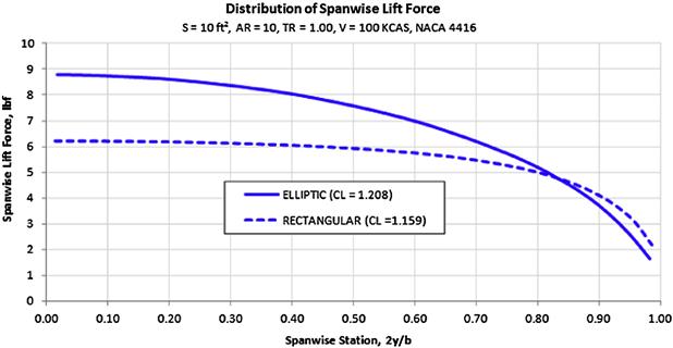


Figure 9-26 shows the distribution of lift as a force along the span. The area under the graph is the shear force along the span and, assuming a cantilevered wing, the progression of integration from tip inboard to root will provide the shear diagram. Then, integrating the shear diagram from tip to root will generate the moment diagram. Note that sometimes this graph is presented using the physical dimensions of the wingspan (e.g. b = 35 ft or similar). In this case, the units for the y-axis of the graph are more correctly represented as lbf/ft (assuming the UK system is being used). Another important observation is the difference in the force generated by the elliptical wing planform when compared to the rectangular form.
Figure 9-27 shows the distribution of section lift coefficients along the span. The advantage of this presentation is that it can be used to evaluate the magnitude of geometric (or aerodynamic) twist required to help control stall progression or even bending moments. Since an airfoil will stall at a specific two-dimensional lift coefficient and this format presents the current two-dimensional lift coefficient (i.e. the section lift coefficient) this can be used to design good stall characteristics into the airplane (see Section 9.6.4, Tailoring the stall progression).
Figure 9-28 shows the distribution of the contribution of the section lift coefficient to the total lift generated by the geometry. It helps demonstrate regions that contribute a lot or little to the overall lift.
9.4.3 Constant-chord (“Hershey-bar”) Planform
Nicknamed for its simple constant-width geometry, this planform is widely used for many different kinds of aircraft, small and large. Light planes that feature Hershey-bar wings include the Beech Model 77 Skipper, Piper PA-38 Tomahawk, Piper PA-28 Cherokee, and Piper J-3 Cub. Among larger aircraft are the de Havilland of Canada DHC-6 Twin Otter and the Shorts 360.
The distribution of spanwise section lift coefficients, Cl, for a Hershey-bar wing is shown in Figure 9-29. This is done for two AOAs; 0° and 10°. For comparison purposes, the latter curve will be superimposed on all subsequent planform shapes so the reader can get a quick glimpse of how the lift distribution of other wing planform shapes differs from that of the constant-chord wing.
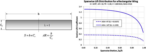
Pros
The configuration has two primary advantages. The first is forgiving stall characteristics, attributed to the reduction in section lift coefficients toward the wingtip (see Figure 9-29). This promotes a very favorable stall progression (growth of flow separation) that begins at the root and moves outboard to the tip, rendering it the last part of the wing to stall. This effect is very desirable as it gives the configuration important roll stability at stall.
The other important advantage is the lower manufacturing costs because all ribs have the same basic geometry and the spar is a constant-thickness beam. This simplicity affects not only the wing ribs and spar, but also the control surfaces.
This configuration is ideal for trainer aircraft or airplanes for which manufacturing cost is imperative.
Cons
Since the wingtip contributes less to the lift generation than the root (in terms of section lift coefficients), the planform is particularly inefficient. For this reason, the planform should never be used for efficient aircraft, such as sailplanes or long-range aircraft. This includes wings and stabilizing surfaces.
9.4.4 Elliptic Planforms
The elliptical wing planform (see Figure 9-30) is most famous for its use in one of the most formidable fighters of the Second World War, the British Supermarine Spitfire. Other aircraft that feature this configuration include: the American Republic P-47 Thunderbolt; and the German Heinkel He-70 He-112B, Mudry CAP-10, and CAP-20. Interestingly, the aerodynamic properties of the planform are widely publicized, even among some laypeople.

The planform shown in Figure 9-30 is a pure ellipse, which means that a straight line extending from tip-to-tip is located at the 50% chord. However, there is no requirement that an elliptic planform has to comply with that geometry. For instance, it would be structurally practical to design it so the quarter-chord was a straight line. This would simplify the design by allowing a straight main spar (albeit with a curved spar height) to be positioned at the quarter-chord.
Elliptical planforms with a straight leading edge or trailing edge (see Figure 9-31) are common on radio-controlled aircraft and sailplanes and are sometimes referred to as crescent-shaped wings. The graph of Figure 9-31 shows that, fundamentally, the distribution of section lift coefficients for the three planform shapes is the same, except at the tip. While all three planform shapes generate a similar total CL at 10°, the one with the straight LE generates a lower section lift coefficient at the tip than the others, implying a less severe washout is required to improve stall characteristics. However, one must be careful in the interpretation of such linear curves because the sharp tip introduces important viscous effects at higher AOAs that render the linear predictions invalid. These are discussed in Section 9.6.3, Deviation from generic stall patterns.
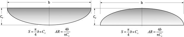
Pros
Its primary advantage is the uniform distribution of section lift coefficients (see Figure 9-30). This distribution makes the planform very efficient when it comes to utilizing the entire span and results in the least amount of lift-induced drag of any planform.
Cons
The planform’s greatest drawback is its producibility, which is severely impaired by the complex compound surfaces. It is very difficult to manufacture using aluminum, as this would call for sheets to be stretched through hydroforming (or similar). However, it is much easier to produce using modern composites.
Another serious drawback is that the section lift coefficients are mostly uniform along the span, which causes the entire wing to stall at once (again assuming a constant airfoil and no washout). This can pose a serious problem for low-speed (or high AOA) operations and requires a decisive washout or airfoil selection to remedy.
9.4.5 Straight Tapered Planforms
A straight tapered wing planform is one for which the root chord is different from the tip chord, such that the smaller chord resides inside two lines that are perpendicular to the plane of symmetry and that are drawn at the LE and TE of the larger chord (see Figure 9-32).
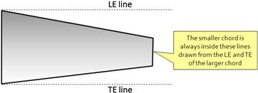
Some authors define straight wings as those that have zero sweep on any spanwise line between 25% and 70% chord. The drawback with that definition is that it excludes common GA aircraft that feature a straight LE or TE.2
The list of airplane types that use this wing planform shape is very long. A generic tapered planform and its spanwise distribution of section lift coefficient is shown in Figure 9-33.
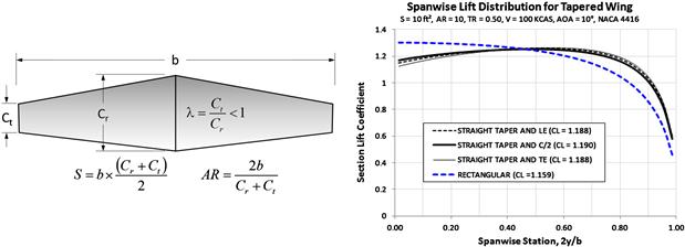
Pros
The primary advantage of tapered wings is reduction in bending moments and lift-induced drag. Straight tapered wings offer improved efficiency over the Hershey-bar wing as the section lift coefficients are higher toward the tip. Consequently, the wingtips contribute more to the total lift coefficient. This, combined with the relative geometric simplicity of the linear taper, which is easier to manufacture than the elliptical planform, renders the planform ideal for most airplanes. The improved efficiency of the configuration usually warrants the increased production complications.
Cons
The taper compromises the stall characteristics and requires a geometric or aerodynamic wing washout, or a combination of both, to be employed. An additional solution might be to select an airfoil for the tip that has a higher stall AOA than the root. It is common to locate root and tip airfoils such that their quarter-chords are on a line perpendicular to the plane of symmetry. This allows a straight main spar to be placed at the quarter-chord of the wing, but this is an effective location as it results in good structural depth that provides the potential for reasonably large fuel tanks behind the spar. The configuration causes manufacturing complications due to the different geometry of each rib.
Straight Leading or Trailing Edges
Other airplanes feature straight tapered wings whose leading or trailing edge is perpendicular to the plane of symmetry (see Figure 9-34). This means that a spanwise line going through the quarter-chord of the root and tip is swept forward or back.

Pros
Improved structural and aerodynamic efficiency over the constant-chord configuration. The straight LE planform may be advantageous if it is foreseen that the operational CG will be too far forward. The opposite holds for an operational CG that turns out to be too far aft.
Cons
It is a drawback that if the wing features a spar that is perpendicular to the plane of symmetry and extends from tip to tip, its caps will be curved. This can be eliminated by sweeping the spar forward, which makes the use of a single-piece spar more challenging.
The hinge line of control surfaces can have a significant forward sweep, which makes them less efficient aerodynamically and can complicate the design of the control system. Among a number of examples of aircraft that feature the straight LE are the Arado Ar-79, Cessna 177 Cardinal, Commonwealth Ca-12 Boomerang, and Fairey Barracuda, and a series of Mooney aircraft feature the planform shape for both the wing and stabilizing surfaces.
On the Mooney aircraft, the straight LE of the horizontal and vertical tails arguably renders them more efficient aerodynamically than the more popular aft-swept tails and, in theory, this allows the tail be a tad smaller, with less wetted area. This is an argument often heard among laypeople. However, an investigation reveals this is not true. Some of that efficiency is simply lost in lowered control authority of the less effective control surfaces whose hinge lines are inevitably swept forward. Of course, the same argument can be made for aft-swept stabilizers – they also have hinge lines that are swept aft. The difference is that the aft sweep adds arm that makes up for the loss in aerodynamic efficiency. A VLM analysis of the Mooney M-20R revealed that its directional stability derivative, Cnβ, is in the range of 0.054 per radian. Introducing a 45° aft sweep in the LE of the VT (no change in surface or wetted area and root chord precisely the same place) increased it to 0.060 per radian, directly contradicting any claims of greater effectiveness of the straight LE tail. This simply means that the reduction in CLα of the VT reduces less than the tail arm increases. The important point is that in the case of the Mooney, the tail is a signature feature for the brand. One can always recognize a Mooney tail and for the brand this is important. But more effective it is not.
Another version of the straight tapered wing is the straight trailing edge planform in Figure 9-34. Many of the same arguments for or against hold for this planform. It is featured on a number of aircraft, among others the Aermacchi MB-326 and MB-339, Bücker Bü-180 Student, Zlin Z-526, 726, and Z-26.
The Compound Tapered Planform
The compound tapered wing planform consists of two tapered sections; the inboard section is an inverse taper and the outboard section has standard taper (see Figure 9-35). The lift distribution for this planform is also shown. It can be seen that section lift coefficients peak inboard, indicating this is where stall would initiate. This is significantly reduced midspan and then increases toward the tip. The analysis indicates the planform is not particularly efficient although the discontinuity at the leading edge may provide some viscous benefits. Among well-known aircraft featuring this planform is the Westland Lysander, a British single-engine observation aircraft with short take-off and landing (STOL) designed in the 1930s. The reason for this choice was pilot visibility – its STOL capability can be attributed to the high-lift system it was equipped with and not the planform itself.
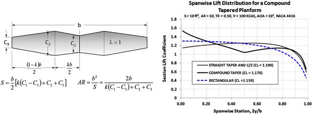
9.4.6 Swept Planforms
Like the tapered wing planform, the swept planform is one of the most common types of geometry found in aviation. Practically all commercial aircraft use swept wings, and even aircraft that operate at low subsonic speeds commonly use the planform shape for their stabilizing surfaces. For this reason, this geometry must be elaborated on in some detail.
The Aft-swept Planform
The invention of the planform is generally thought to date back to the 1930s. However, it was not possible without the work of scientists who preceded the era. Meier [11] takes this history back to Isaac Newton (1643–1727), Pierre-Simon, Marquis de Laplace (1749–1827), Ernst Mach (1838–1916), and many others, up to Adolf Busemann (1901–1986), who is generally credited with the invention of the swept-back wing. Busemann belonged to a group of very famous German scientists who were led by Ludwig Prandtl (1875–1953). The best known were Theodore von Kármán (1881–1963), Max M. Munk (1890–1986), and Jakob Ackeret (1898–1981) [12]. The result of Busemann’s work was first published at the 5th Volta conference in Rome in 1935 [13]. The Volta conference was an annual conference of physics, mathematics, history, and philosophy, named to honor the great Italian physicist Alessandro Volta (1745–1827). In the USA, Robert T. Jones tested swept-back wings toward the end of 1944. It was the first such work in the USA. It was published in 1945 in NACA TR-863 [14]. In it, Jones cites Busemann’s research from 1935 as one of his references.
Pros
One of the primary advantages of the configuration is that when used with high-speed aircraft, it delays the formation of shockwaves to a higher Mach number (see Section 9.3.3, Leading edge and quarter chord sweep Angles, ΛLE and ΛC/4).
The aft-swept configuration is less susceptible to flutter than either the straight or the forward-swept configurations. This results from the tendency of a positive (vertical upward) lift force to reduce the AOA of the tip through aeroelastic effects.
The aft-swept (or forward-swept) configuration is also a possible solution when the CG is expected to end up too far aft or forward on a proposed configuration. The Messerschmitt Me-262 Schwalbe was the first jet aircraft to feature a swept-back wing. However, the modest sweep angle of 18.5° was insufficient to greatly impact divergence drag number and was a consequence of its Junkers Jumo jet engines being heavier than expected. For this reason its originally straight wings were swept aft to solve an issue with the location of its center of gravity [15].
Cons
Among drawbacks is the deterioration of airflow close to the tip of the planform with an increase in AOA. The reason for this deterioration is explained in Section 9.6.5, Cause of spanwise flow for a swept-back wing planform. Two important consequences of this phenomenon is a powerful nose pitch-up moment that develops as the AOA approaches stall and an accompanying deterioration in roll stability and aileron effectiveness.
Since the center of lift is positioned behind the wing root attachment there is an increase in wing torsion, often substantial, that increases the weight of the airframe.
The configuration is more susceptible to control reversal as a result of the tendency of the lift force to reduce the AOA of the tip through aeroelastic effects. The same effect moves the center of lift forward with AOA if the wing is flexible and regardless of flexibility when the wing stalls. It is the cause of the powerful and dangerous nose pitch-up moment at stall.
Aircraft with swept wings often experience issues with the wing fuel tanks. For instance, as the airplane rotates to take-off and begins to climb, fuel will flow toward the outboard and aft side of the tank. This may cause the CG to shift aft. This is solved using so-called baffle check valves, which are one-way flapper valves that allow fuel only to flow inboard [16]. Large transport aircraft, some carrying as much as 40% of their gross weight in fuel, can experience large changes in CG location as fuel is consumed. This often calls for a computer-controlled fuel management system that monitors and controls how fuel from the wing tanks is used.
In order to understand the advantages and disadvantages of the swept aft configuration, it is helpful to break it down depending on taper ratio, λ. This way it is possible to consider three classes; λ < 1, λ = 1, λ > 1 (see Figure 9-36 and Figure 9-37). Most aircraft with aft-swept wings fall into the first category. In fact, there as so many different types of aircraft in this class that it would be unfair to name any particular one. Almost all high-speed military and passenger transport aircraft feature the configuration. These are particularly easy to locate.

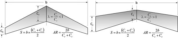
The other two classes contain considerably fewer members. When it comes to the second class, for which λ = 1, there is a handful of examples. In current times, the Boeing B-2 Spirit is probably the best known. However, there are others. Among those are the Dunne Monoplane and Biplane, designed in the 1910s by John W. Dunne (1875–1949). The English Electric Lightning, MiG-8 Outcka, MiG I-320, MiG-17, Sukhoï Su-15P, and Yakovlev Yak-25 (Flashlight) have a λ close to 1. And in the third category, the Republic XF-91 Thunderceptor is the only contender. Designed with the tip chord larger than the root chord, the idea was to reduce the section lift coefficients at the tip in order to improve low-speed handling.
The Forward-swept Planform
One of the aerodynamic advantages of the forward-swept wing can be seen in Figure 9-38: the reduced section lift coefficients at the tip. The distribution ensures the inboard wing stalls first and gives the configuration great roll stability at stall (remember this also means while pulling high gs), making it almost impossible to tip stall. The reduced tip loading also means that the ailerons retain far more authority at high AOA than on an aft-swept configuration. This improves controllability during critical phases of the flight, such as during landing. The shape of the lift distribution places the center of lift closer to the plane of symmetry, reducing bending moments (although it does not prevent divergent torsional tendency). Additionally, spanwise flow is directed inboard rather than outboard, where the fuselage more or less acts like an endplate or a fence that prevents early separation.
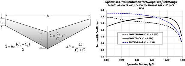
FIGURE 9-38 Basic geometry and basic lifting characteristics of the forward-swept wing, compared to the constant-chord and the tapered swept-back planform shapes.
The primary disadvantage of the geometry is divergent aeroelastic deformation. As the AOA of the wing is increased, the elastic torsional deformation twists the wing, increasing the AOA further. Forward-swept wings must be especially reinforced to keep the divergent deformation to a minimum, inevitably increasing their weight.
The first major development of a forward-swept wing configuration was the German Junker Ju-287. An interesting discussion of its development is given in Ref. [11]. The configuration has been used in a few other designs, including the Grumman X-29, the HFB-340 Hansajet, and the Sukhoi Su-47. A modest forward sweep is relatively common, for instance in sailplanes and a number of GA aircraft. However, it is almost always a solution to a CG problem and not for compressibility fixes.
Variable Swept Planform
The variable sweep planform (see schematic in Figure 9-39) dates back to the German Messerschmitt P.1101, whose incomplete prototype was discovered at the end of WWII. It featured a swiveling wing design whose sweep angle was to be selected and set manually before each flight. Later, this innovative design led to fighter and bomber models, such as the General Dynamics F-111, Grumman F-14, Sukhoi Su-17, Panavia Tornado, and others. The configuration is not used in any GA aircraft, as it inevitably leads to a heavier airframe, control system complexity, and other complications. It is really a configuration suited for supersonic aircraft, where it solves problems at the high- and low-speed extremes of the flight envelope. It is included here for the sake of completion.
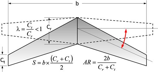
9.4.7 Cranked Planforms
The term “cranked” refers to a break in the leading or trailing edge of a wing that changes the leading (or trailing) edge sweep angle. It turns out that such planform shapes are surprisingly common – for instance a large number of Cessna single-engine aircraft feature cranked wings, as do other popular aircraft such as the Piper PA-28 Cherokee Archer or the Beechcraft Bonanza. Although included in a separate class, the double delta configuration is also technically a cranked planform. In fact, any aircraft that features a leading edge extension falls into this category. However, by convention, double deltas are considered a member of delta wings. Regardless, this class is inclusive and includes a number of wing planform shapes that otherwise might be considered unrelated.
Semi-tapered Planform
The semi-tapered planform is one that has a constant-chord inboard section and a tapered outboard section (see Figure 9-40). The planform increases the section lift coefficients on the outboard wing and improves its efficiency over that of the Hershey-bar wing. A side benefit of this is improvement in aileron effectiveness. The drawback is the added complexity of construction, and reduction in the aileron effectiveness if its hingeline becomes highly swept.
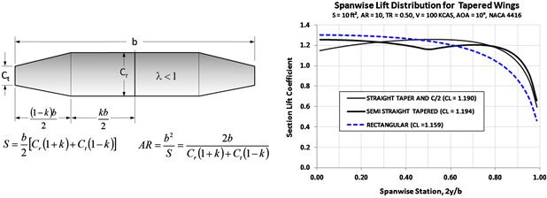
FIGURE 9-40 Basic geometry and lifting characteristics of the semi-tapered wing, compared to the constant-chord and the tapered swept-back planform.
The configuration is best known on a family of single-engine Cessna aircraft: the 150, 152, 172, 182, 206, and many others. It is also used on a number of Piper PA-28 Warrior and Cherokee Archer aircraft.
Crescent Planform
The crescent wing planform (Figure 9-41) has seen very limited use. It is best known for its use on the British Handley-Page Victor, where the highly swept inboard section of the wing allowed the use of a thick airfoil without introducing early shock formation at high Mach numbers. The thick airfoil was needed to accommodate its four jet engines, which were buried in the wing root. The wing of the Victor varied in quarter-chord sweep and thickness, progressively from 22° and 4% t/c at the tip to 53° and 16% at the root. This allowed a constant Mcrit to be maintained along the wing and resulted in more efficient reaction of bending moments. A consequence of this geometry was improved aileron control authority and reduced tendency for tip stall and subsequent nose pitch-up.

Schuemann Planform
The Schuemann planform shape has already been thoroughly introduced in the Appendix C1.5.2, The Schuemann wing. It is featured on a number of sailplanes, for instance, the Stemme S-10 and the DG-1000. The wing style has also been introduced on commuter aircraft such as the Dornier Do-228, Dornier 328, and Fairchild-Dornier 328JET.
Figure 9-42 shows the fundamental dimensions of the planform shape and the distribution of the section lift coefficients compared to those of a Hershey-bar and elliptical planform shapes. It can be seen that the distribution approximates that of the elliptical planform, leading to a reduction in lift-induced drag. This explains the wing’s popularity for sailplanes. The figure also reveals that a potential problem with the wing is an early wing tip stall, not unlike the elliptical wing and is caused by the sharp outboard taper. This is of course complicated by viscous effects at the wingtip, as highly swept wingtips may position the tip vortex so it suppresses early tip stall tendency, not unlike delta wings. Sailplane wingtips at a high AOA will flex substantially due to aeroelastic effects. This effectively unloads the wingtip and loads up the center portion of the wing, which then stalls before the wingtip. For this reason, sailplanes usually have good stall characteristics. A short and stiff wing, likelier to be used for a GA aircraft, will not flex nearly as much as the high AR wing and should thus be expected to feature decisive wing washout at the tip, unless the tip segment of the wing features a high enough sweep.
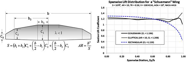
9.4.8 Delta Planforms
The Delta Planform Shape3
A discussion of the pros and cons of delta wings (see schematic in Figure 9-43) is given in Appendix C1.5.5, The delta wing, and will not be elaborated on here, other than that they are planform shapes intended for high-subsonic or supersonic aircraft and not low-subsonic airplanes. Even though it is certainly possible to use delta wings for low-speed airplanes (as evident by the Dyke Delta) it is a choice that is hard to justify for reasons other than fun flying; with reduced storage space (thanks to a short wingspan), being another drawback. Deltas stall at very high angles of attack and generate low CLmax compared to straight un-swept wings; they will therefore require high approach speed and deck angles. As an example, the 2000 lbf Dyke JD-2 Delta reportedly stalls at about 61–65 KCAS [17]. This means that the 173 ft2 wing area generates a CLmax around 0.8–0.9. That is 50–65% less than conventional straight wings. They also have poor LDmax, which is of concern for engine-out emergencies. The best-known aircraft that uses the configuration is the Dassault Mirage III and its various derivative aircraft (e.g. Mirage IV, 2000, Rafale).
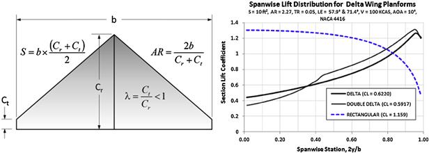
The Double-delta Planform Shape
The double delta (see Figure 9-44) is also known as the compound delta. They have an advantage over conventional delta wings in that they produce a vortex pair, rather than a single vortex over each wing that mutually interfere with each other. The resulting system increases the lift of the double delta over that of the conventional delta, rendering supersonic fighter aircraft far more maneuverable [18]. When it comes to subsonic aircraft, the configuration suffers from similar limitations to the single delta. The configuration has been used on military aircraft like the SAAB J-35 Draken and General Dynamics F-16E cranked arrow.
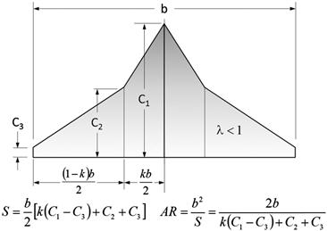
9.4.9 Some Exotic Planform Shapes
Disc- or Circular-shaped Planform
In short, the disc-shaped planform (see Figure 9-45) is something no self-respecting aircraft designer should propose as a primary lifting surface. Perhaps inspired by the fad of UFO sightings in the 1950s, the well-respected but long-defunct Avro Canada Ltd, a company that at one time employed some 50,000 people, dared to develop the AVRO Canada VZ-9A, nicknamed the AVRO car. A secret military project, the Avrocar employed the Coandǎ effect to generate lift and thrust. The project was cancelled in 1961 when it became clear that insufficient thrust and stability issues would hamper its success.

Figure 9-45 shows a comparison of spanwise lift distribution between the disc planform and an elliptical and a Hershey-bar wing. In spite of the uniform distribution of section lift coefficients, the graph clearly shows how inefficient this planform shape is when compared to the Hershey-bar or elliptical wings; it barely ekes out one-third of the lift at the selected AOA (10°). From an efficiency standpoint, the disc-shaped wing is simply beyond objectionable. However, it is presented here as it is an ideal shape for a radar disc of the kind installed on a reconnaissance or early warning and control system (AWACS) military aircraft such as the Boeing E-3 Sentry (a modified Boeing 707) or Grumman E-2 Hawkeye. For such applications a shallow lift curve slope is essential for stability and control reasons.
Other Configurations
Four other configurations are shown in Figure 9-46: an ogival, joined wing, blended wing-body, and a rhomboid planform. Lift distribution curves for these shapes will not be presented here, since these planform shapes are highly specialized or experimental.
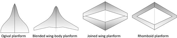
9.5 Lift and Moment Characteristics of a 3D Wing
As has already been thoroughly discussed, lift, drag, and pitching moment are almost always converted into a dimensionless coefficient form as this allows transferability (see Equation [8-8]). The lift, drag, and pitching moment coefficients are defined as shown below (note the capitalization of the forces and moments for the three-dimensional object):
 (9-47)
where the variables have already been defined elsewhere (e.g. see Variables at the end of this chapter).
In this section, the three-dimensional lift and moment characteristics of the wing will be evaluated, whereas drag is treated in Chapter 15, Aircraft drag analysis. Here, a number of important characteristics will be discussed, including construction of the three-dimensional lift curve, estimation of span efficiency and the maximum three-dimensional lift coefficient, stall behavior, tailoring of stall characteristics, and others.
9.5.1 Properties of the Three-dimensional Lift Curve
Figure 9-47 shows a typical three-dimensional lift curve. Overall, the curve displays identical characteristics to that of the two-dimensional curve of Section 8.1.4, Properties of typical airfoils, except it represents the behavior of the entire aircraft (wings, fuselage, HT, etc.). The contribution of the individual components of the aircraft to the overall non-linear shape of the curve may make it very different from that of the selected airfoils. As before, the aircraft designer is most interested in the following characteristics:

Lift Curve Slope, CLα
The lift curve slope is a measure of how rapidly the wing generates lift with change in AOA. As stated in Section 8.1.4, the theoretical maximum is 2π, although real airfoils deviate from it. The lift curve slope of a three-dimensional wing is always less than that of the airfoils it features (see Section 9.5.3, Determination of lift curve slope, CLα, for a 3D lifting surface). Once a certain AOA has been achieved the wing will display a pronounced reduction in the lift curve slope (see Figure 9-47). This point is called stall and, although not shown in the figure, occurs both at a positive and negative angle-of-attack. The lift at stall dictates how much wing area the aircraft must feature for a desired stalling speed.
Maximum and Minimum Lift Coefficients, CLmax and CLmin
The largest and smallest magnitudes of the lift coefficient are denoted by CLmax and CLmin, respectively. It indicates at what angle-of-attack the airplane will achieve its minimum airspeed (stalling speed), or what wing area is required for a desired stalling speed. As for the airfoil, the stall is defined as the flow conditions that follow the first lift curve peak, which is where the CLmax (or CLmin) occur (see, for instance, Ref. [19]). Both values are required when generating aerodynamic loads for the structures group.
CL at Zero AOA, CLo
CLo is the value of the lift coefficient of the wing at zero AOA. It is of great importance in the scheme of things, because it affects the angle-of-incidence at which the wing must be mounted. Generally this value ranges from 0.0 (for symmetric airfoils) to 0.6 (for highly cambered airfoils). It is negative for under-cambered airfoils (e.g. airfoils used near the root of high subsonic jet aircraft).
Angle-of-attack at Zero Lift, αZL
This is the angle at which the wing generates no lift. For positively cambered airfoils this angle is always negative, unless some specific components (e.g. cambered fuselage) affect it greatly. For symmetrical airfoils it is always 0°.
Linear Range
The linear range is analogous to that of the airfoil, except it applies to the entire aircraft. In this range, the following equation of a line can be used to describe how lift varies with AOA.
![]() (9-48)
(9-48)
Angle-of-attack where Lift Curve Becomes Non-linear, αNL
Once a certain AOA is reached the wing begins to display a pronounced reduction in the lift curve slope. This always happens before the stall AOA is reached.
Angle-of-attack for Maximum Lift Coefficient, αstall
Once a certain AOA is reached, a pronounced reduction in lift curve takes place; this is the stall.
Design Lift Coefficient, CLC
The design lift coefficient is the CL at which the aircraft is expected to operate during the mission for which it is designed. This is usually the lift coefficient during cruise. It is important to select an airfoil that has been designed to generate the least amount of drag at that lift coefficient (see Section 8.3.15, Airfoil selection how-to), as well as ensure flow separation areas are completely suppressed for minimum drag. In the case of a constant cruising speed (or loiter) mission, if the target airspeed is known, it is possible to estimate this design cruising speed using the weight of the airplane at the beginning and end of the mission using the following expression:
![]() (9-49)
(9-49)
where
Angle-of-attack for Design Lift Coefficient, αC
Ideally, the airplane should be flying at an AOA that generates the least amount of drag during the intended mission for which it is designed. For instance, this could be a cruise or long-range performance point. In the case of the design mission being a cruise or loiter mission, this AOA can be calculated from Equation (9-43).