
Performance – Introduction
Abstract
Methodologies to model the atmosphere are provided, but this is a prerequisite to any performance analyses. This modeling uses the US Standard Atmosphere, published by NOAA, NASA, and USAF. Methods to estimate atmospheric properties up to 36,089 ft (11,000 m) are presented, with methods for altitudes up to 278,000 ft (85 km) detailed in appendix A. This is followed by methods to calculate true airspeed, equivalent airspeed, and other important airspeeds. Then, a step-by-step procedure to create a V-n diagram is presented, with a corresponding discussion of the FARs that requires its generation. Finally, two sample aircraft that are used to demonstrate performance calculations in other chapters are presented. These are the Cirrus SR22 and the Learjet 45XR.
Keywords
Performance padding; atmosphere; pressure; density; temperature; altitude; density altitude; pressure altitude; standard atmosphere; lapse rate; humidity; airspeed; true airspeed; calibrated; airspeed; ground speed; equivalent airspeed; indicated airspeed; speed of sound; Mach number; flight envelope; maneuvering load; gust load; maneuvering speed; stall speed; dive speed; cruising speed; 14 CFR Part 23; SR22; Learjet 45XR
Outline
16.1.1 The Content of this Chapter
16.1.2 Performance Padding Policy
16.2.1 Atmospheric Ambient Temperature
16.2.2 Atmospheric Pressure and Density for Altitudes below 36,089 ft (11,000 m)
16.2.3 Atmospheric Property Ratios
16.2.4 Pressure and Density Altitudes below 36,089 ft (11,000 m)
16.2.5 Density of Air Deviations from a Standard Atmosphere
Change in Density Due to Humidity
16.2.6 Frequently Used Formulas for a Standard Atmosphere
16.3.1 Airspeed Indication Systems
16.3.2 Airspeeds: Instrument, Calibrated, Equivalent, True, and Ground
16.3.3 Important Airspeeds for Aircraft Design and Operation
16.4.1 Step-by-Step: Maneuvering Loads and Design Airspeeds
Step 1: Establish Load Factors n+ and n−
Step 2: Design Cruising Speed, VC
Step 4: Design Maneuvering Speed, VA
Step 5: Design Speed for Maximum Gust Intensity, VB
Step 6: Set Up the Initial Diagram
16.4.2 Step-by-Step: Gust Loads
Step 7: Calculated Gust-related Parameters
Step 8: Calculate Gust Load Factor as a Function of Airspeed
Step 9: Calculate Gust Load Factor as a Function of Airspeed
Step 10: Finalize Gust Diagram
Convenient Relations to Determine Location of Intersections
16.4.3 Step-by-Step: Completing the Flight Envelope
V-n Diagrams with Deployed High-lift Devices
16.1 Introduction
Any flight can be split into a number of phases that are clearly distinct by their nature. These are the take-off, climb, cruise, descent, and landing. In addition to these, there are a large number of maneuvers performed while airborne that involve acceleration of one kind or another; for instance, turning flight, rolls, loops, and many others. The purpose of the next six chapters is to present aircraft performance theory in a systematic manner intended to be particularly helpful to the aircraft designer. The titles of these chapters are in an order of occurrence during the flight:
A proper prediction of aircraft performance is another extremely important step in the entire design process. Performance and payload are what sell an aircraft more than anything else. The same scenario holds here as for the estimation of weight and drag – an erroneous prediction will manifest itself as soon as the aircraft takes off for the first time and can devastate a development program, if not cancel it altogether.
This section serves as a prologue to the performance methods. Here, topics that apply to all the performance methods, such as types of airspeed and the atmospheric model, will be presented. It will also introduce a couple of example aircraft to be used in the subsequent chapters. The methods presented here are proven and standard in the industry. However, there are important limitations that must be brought up. The quality of the drag model weighs the most. The aspiring aircraft designer is advised to acquire experience with these methods by applying them to existing aircraft for which performance data has been published. This will build experience and an understanding of their accuracy that serves well when assessing the performance of new designs.
As discussed in Chapter 15, Aircraft Drag Analysis, there are typically three drag models: the simplified, adjusted, and non-quadratic. The first two models assume the induced drag can be represented in terms of the lift coefficient squared (they are quadratic). Both become inaccurate at high AOAs, in particular the simplified model and therefore, generally, it should be avoided. The non-quadratic is typically used to evaluate the performance of sailplanes, as they feature a drag bucket that cannot be described by the quadratic models.
The simplified drag model is only usable for aircraft whose CLminD is zero. This is rare as most airplanes use cambered airfoils. Some fighter aircraft and aerobatic aircraft are designed with airfoils that have a very small camber or are fully symmetrical. Such airplanes may have CLminD = 0, although the geometry of their fuselages may shift their drag polars, rendering a non-zero CLminD. The non-quadratic drag model, on the other hand, must usually be represented in the form of a lookup table. The performance methods presented will work equally with all the models, although the accuracy of the predictions will depend on the selected model. The reader should keep in mind that subsequent sections will invariably use the simplified drag model to present a close-form expression of performance concepts. The primary advantage of the simplified drag model is that it allows for clear and concise formulation, which is much harder to accomplish using the adjusted or non-quadratic drag models. Several methods will also derive expressions using the adjusted drag model.
16.1.1 The Content of this Chapter
• Section 16.2 presents a description of how to model the atmosphere.
• Section 16.3 presents methods to calculate true airspeed, equivalent airspeed, and other important airspeeds.
• Section 16.4 presents the V-n diagram and shows how to create it.
• Section 16.5 presents two sample aircraft that will be used to demonstrate performance calculations: the Cirrus SR22 and the Learjet 45XR.
16.1.2 Performance Padding Policy
Performance information constitutes a very sensitive portion of the aircraft development. It is important for the design team to recognize that performance predictions released internally can be used in both a constructive and a deconstructive manner. One concern is that if the marketing department gets their hands on such predictions, they will use it to sell airplanes that have yet to be built and flown. Of course, selling airplanes is very desirable; however, to the marketing people, a predicted cruising speed of 276 KTAS means a real cruising speed of 276 KTAS. On the other hand, to the performance analyst who understands the shortcomings of the predictions, this cruising speed means a possible 270 to 276 KTAS. All of this is fine, unless of course the airplane turns out to be capable of 270 KTAS, or worse yet, only 265 KTAS. Then, the manufacturer will have to spend considerable effort and loss of revenue pleasing unhappy customers who were promised a new airplane capable of 276 KTAS.
To prevent such annoyances, many businesses require conservatism in prediction through padding factors. The cognizant design lead is urged to consider such factors and ensure the performance prediction team establishes a padding policy that enjoys a need-to-know-only status (i.e. no one outside the Aero group knows the actual padding factors). So, if the predicted cruising speed is 276 KTAS, then marketing is told 272 KTAS, or some other reasonable figure. The purpose is not deceit but financial protection.
Additionally, disclosure of performance information should be done with care, because the information can hurt the competitive edge of the company. For instance, an ill-tempered test pilot shouting something along the lines of “the darn thing barely climbs” in a moment of frustration may be echoed elsewhere, perhaps by a careless technician who happened to overhear the pilot. He or she might be unaware that the airplane was being tested with deployed landing gear, at gross weight, and at a high-density altitude. Something as seemingly innocent as that can easily start a rumor that is used by a competitor against the developer.
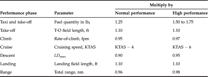
Table 16-1 shows recommended padding factors for normal and high-performance GA aircraft. As an example of how it is used, consider an aircraft whose T-O field length has been predicted to be 1200 ft. The table suggests the performance team should report 1320 ft.
16.2 Atmospheric Modeling
Atmospheric modeling is the determination of the properties of air in which an airplane is operated. The properties are outside air temperature, pressure, density, and viscosity. The ability to accurately quantify them is absolutely imperative for the evaluation of the large number of aerodynamic characteristics of an airplane. Our understanding of the atmosphere is extensive, although it is by no means complete. Among important discoveries is that the atmosphere is stratified. The most active layer is the one closest to ground level; the troposphere. While most aircraft operate in this layer, flying above it is becoming more common. Atmospheric science has also revealed there can be substantial wind speeds in the layers above the troposphere. The current altitude record set by an aircraft is held by a modified Russian MiG-25 fighter aircraft, which on August 31, 1977, climbed to an estimated altitude of 123,524 ft (37.65 km) [1]. In August 2001, an unmanned experimental solar-powered aircraft, aptly named Helios, designed and built by NASA, climbed to an altitude of 96,863 ft (31.78 km) [2], an official world record altitude for a propeller-powered aircraft. In June 2003, the aircraft broke up in midair after an encounter with atmospheric turbulence (Accident report is available from Ref. [3]).
A detailed atmospheric model, based on document US Standard Atmosphere 1976, published by NOAA (National Oceanic and Atmospheric Administration), NASA (National Aeronautics and Space Administration), and the US Air Force, extending up to approximately 85 km (280,000 ft) is provided in Appendix A, Atmospheric modeling. The reader is directed toward the appendix for information regarding the higher altitudes, as well as a Visual Basic for Applications code intended for use with Microsoft Excel, which calculates the aforementioned properties with ease. In the interests of space, only fundamental equations needed to obtain temperature, pressure, and density in the troposphere are provided in this section. All derivations are provided in the appendix. The reader is well advised to review the appendix as it contains a large number of very useful equations intended to estimate other properties of the atmosphere, as well as deviations from standard atmosphere.
16.2.1 Atmospheric Ambient Temperature
Let’s start by considering the temperature; T. Change in air temperature with altitude can be approximated using a linear function:
![]() (16-1)
(16-1)
An alternative form of Equation (16-1) is:
![]() (16-2)
(16-2)
where
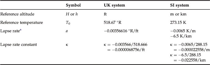
In the world of aviation T is usually referred to as the “outside air temperature” or “ambient temperature.” Practically all aircraft operate inside the altitude band ranging from S-L to 11,000 m (36,089 ft). That part of the atmosphere is, thus, of considerable interest to us. The variables to be used with the above equations in that band are summarized in Table 16-2.
TABLE 16-2
Common Temperature Constants in the Troposphere
a“The rate at which air cools or warms depends on the moisture status of the air. If the air is dry, the rate of temperature change is 1 °C/100 meters and is called the dry adiabatic rate (DAR). If the air is saturated, the rate of temperature change is 0.6 °C/100 meters and is called the saturated adiabatic rate (SAR). The DAR is a constant value, that is, it’s always 1 °C/100 meters. The SAR varies somewhat with how much moisture is in the air, but we’ll assume it to be a constant value here. The reason for the difference in the two rates is due to the liberation of latent heat as a result of condensation. As saturated air rises and cools, condensation takes place. Recall that as water vapor condenses, latent heat is released. This heat is transferred into the other molecules of air inside the parcel causing a reduction in the rate of cooling” [4].
Note that the author prefers to write the constants explicitly, rather than in the scientific format (e.g. −6.8756 × 10⁻⁶) because it is simply faster to enter using calculators. The author recognizes that this may annoy some readers and empathizes if this is the case. On the flipside, using the scientific format for a number with only five zeros can be annoying and therefore the author uses the scientific format for six or more zeros. The following mnemonic will help you remember the number of zeros when entering the lapse rate constant. Say “one zero, two zeros, three zeros” while typing ‘0.’, ‘00’, ‘000’. Then enter ‘68756.’
16.2.2 Atmospheric Pressure and Density for Altitudes below 36,089 ft (11,000 m)
The hydrostatic equilibrium equations allow the pressure, p, and density, ρ, to be calculated as functions of altitude, h, as follows:
![]() (16-3)
(16-3)
![]() (16-4)
(16-4)
where
κ = lapse rate constant, which is obtained from Table 16-2
16.2.3 Atmospheric Property Ratios
The pressure, density, and temperature often appear in formulation as fractions of their baseline values. Consequently, they are identified using special characters and are called pressure ratio, density ratio, and temperature ratio.
![]() (16-5)
(16-5)
![]() (16-6)
(16-6)
![]() (16-7)
(16-7)
16.2.4 Pressure and Density Altitudes below 36,089 ft (11,000 m)
Sometimes the pressure or density ratios are known for one reason or another. It is then possible to determine the altitudes to which they correspond. For instance, if the pressure ratio is known, we can calculate the altitude to which it corresponds. The altitude is then called pressure altitude. Similarly, from the density ratio we can determine the density altitude.
![]() (16-8)
(16-8)
![]() (16-9)
(16-9)
16.2.5 Density of Air Deviations from a Standard Atmosphere
Atmospheric conditions often deviate from the models shown above. Often it is because the atmospheric temperature differs from the average temperature, due to meteorological conditions. Such deviations can be handled using the equation of state ρ = p/RT, and calculating the pressure using Equation (16-3) and introducing the temperature deviation directly. This is reflected below, using the UK system:
![]() (16-10)
(16-10)
where
T = standard day temperature at the given altitude per the International Standard Atmosphere in °R At S-L it would be 518.67 °R, at 10,000 ft it would be 483 °R, and so on
ΔTISA = deviation from the International Standard Atmosphere in °F or °R
![]() (16-11)
(16-11)
where
T = standard day temperature at the given altitude per the International Standard Atmosphere, in degrees K. At S-L it would be 288.15 K, at 10,000 ft it would be 483 °R, and so on
ΔTISA = deviation from the International Standard Atmosphere in K or C
For non-standard atmosphere, use a negative sign for colder and a positive sign for warmer than ISA for ΔTISA.
EXAMPLE 16-2
Determine the density of air at 8500 ft on a day that is 30 °F colder and then 30 F hotter than a standard day.
Solution
First, determine the ISA temperature at 8500 ft using the value of κ = −0.0000068756/ft (from Table 16-3):

![]()
Then, “plug and chug” into Equation (16-10):
![]()
![]()
These are 6.5% greater and 5.8% lighter than standard day density (0.001840 slugs/ft3), respectively.
Change in Density Due to Humidity
In addition to temperature, humidity also affects density. Under certain circumstances, it may be necessary to account for this phenomenon when estimating aircraft performance – in particular T-O and landing performance. This section presents a method to account for humidity. Humidity is the amount of water vapor present in air. Humidity is typically expressed using any of the following methods:
• Absolute humidity, which is the mass of water vapor per unit volume of air. It is presented as a dimensionless number.
• Relative humidity, which is the ratio of the water vapor pressure present in air to the vapor pressure that would saturate it [5] (and cause precipitation) – if 1.00 (or 100%), precipitation will occur. This is what is usually reported by weather forecasters on TV.
• Specific humidity, which is the mass of water vapor per unit mass of air, including the water vapor – usually expressed as grams of H2O per kilogram of air. Also referred to as humidity ratio.
As a rule of thumb, the density of dry air is higher than that of humid air. The presence of water molecules in air displaces the oxygen and nitrogen atoms so their amount per unit volume decreases. As a consequence, the mass of a unit volume of the humid air decreases and the density is reduced. A general expression for the density of moist air is given below:
![]() (16-12)
(16-12)
where
ρstd = density at altitude, calculated by standard methods
R = specific gas constant for air, see Table 16-3
RH2O = specific gas constant for water vapor, see Table 16-3
Humidity is commonly represented using relative humidity (RH), presented as a percentage (e.g. 50% humidity). If the ambient temperature is known in °C, this can be converted into a humidity ratio using the following relation:
![]() (16-13)
(16-13)
16.2.6 Frequently Used Formulas for a Standard Atmosphere
For convenience, the equations for temperature, pressure, and density are summarized below for a standard atmosphere for both the SI and UK systems of units by inserting the appropriate constants. Note that the subscripts represent the units for each value.
Temperature in degrees Rankine and Fahrenheit (h is in ft):
![]() (16-14)
(16-14)
Temperature in degrees Kelvin and Celsius (h is in m):
![]() (16-15)
(16-15)
Pressure in psf and psi (h is in ft):
![]() (16-16)
(16-16)
Pressure in Pa and mbar (h is in m):
![]() (16-17)
(16-17)
Density in slugs/ft3 (h is in ft):
![]() (16-18)
(16-18)
![]() (16-19)
(16-19)
![]()
![]()
![]() (16-20)
(16-20)
![]() (16-21)
(16-21)
![]() (16-22)
(16-22)
16.3 The Nature of Airspeed
Arguably, the airspeed indicator (ASI) is the most important instrument in any aircraft. This is because the pilot operates the airplane based on the airspeed. He or she base their decision to deflect the elevator to lift off the runway when the airplane has accelerated to a specific airspeed, knowing that once airborne they must maintain a specific airspeed in order to maximize either the rate of climb or the angle of climb. The pilot knows that he or she must maintain airspeed higher than the stalling speed and that they must establish and maintain a specific airspeed during cruise, based on intent to maximize range, endurance, or simply comply with a direction set by air traffic controllers. And the pilot knows that he or she must maintain a specific airspeed during descent. The ASI also tells the pilot when it is safe to retract or deploy the landing gear or flaps, and how best to perform approach to landing. Practically all maneuvering is based on the airspeed at which the airplane is flying. No other instrument is used quite like the ASI.
This section focuses on the airspeed. It details how to determine the number of types of airspeed that are of importance to designers and pilots alike, such as true airspeed, calibrated airspeed and others. And it defines specific airspeeds that are important from a regulatory and operational angle – the V-speeds.
16.3.1 Airspeed Indication Systems
Pilots are often overheard talking about the various V-speeds. This is not some jargon that is limited to the pilot community, but rather it originates with engineers in the aviation industry. The term V-speeds denotes nothing but common symbols for types of airspeeds that are important when describing the capabilities of an aircraft. It is imperative to be familiar with these terms.
Figure 16-1 shows the dial of a typical analog airspeed indicator (ASI). The one shown presents the airspeed using units of knots (KIAS). Some airspeed indicators show the airspeed in miles per hour or kilometers per hour. However, units of knots and ft/s are exclusively used in this book. It is imperative to convert all important airspeeds to knots, as this is the unit of airspeed most widely used in the world of aviation. Also, a number of noticeable markings are shown, but these have a specific meaning described in the figure. Pilots are trained to operate the aircraft using these airspeeds. The airspeeds are discussed in greater detail elsewhere in the text.

Modern aircraft feature computer-drawn airspeed indicators that are displayed on special monitors called the primary flight display (PFD). These allow for sophisticated depiction of information for the pilot, all but eliminating the need for guess work when operating the aircraft. The PFD shown in Figure 16-2 is an example of a typical such screen in a modern passenger jet. Among others, the device directly relays to the pilot the calibrated airspeed (VCAS), Mach number (M), and ground speed (GS), which in Figure 16-2 can be seen to amount to 262 KCAS, 0.792, and 381 KGS, respectively. It also displays high and low speed limitations. For instance, the VMO/MMO limitations can be seen as the thick dotted ribbon extending from 285 KCAS and upward. The thin lined ribbon extending from 275 to 285 KCAS indicates the maximum maneuvering speed, which typically provides a 1.3 g margin for maneuvering. This means that the pilot can increase the speed by that amount, which would be required to maintain a level 40° bank angle at that altitude. The thin lined ribbon extending from the bottom to approximately 249 KCAS indicates that the airplane’s stick shaker is activated. Some of these values are weight dependent and are determined in real time by the airplane's flight computer system.
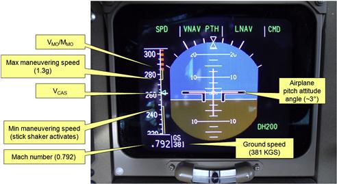
FIGURE 16-2 Markings of a modern airspeed indicator shown on a primary flight display (PFD). (Photo by Gudbjartur Runarsson)
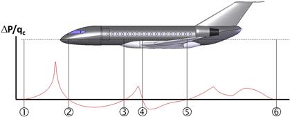
An airspeed indicator needs two pressure sources: dynamic pressure and atmospheric. The dynamic pressure is obtained using a pressure probe called a pitot tube or simply a pitot (pronounced pee-toh). The pitot tube has an opening that faces the flow direction and senses stagnation pressure. The atmospheric pressure probe, called a static source, is oriented perpendicular to the flow direction. It senses static pressure. Then the ASI displays the airspeed based on the difference between the two pressure sources. Of the two, measuring the static pressure is far more difficult than the dynamic pressure. The static source is typically located on the fuselage, although other locations are certainly possible. If installed on a fuselage, we would ideally like to install the static source in a location where the pressure equals the static pressure in the far-field, at all AOAs and airspeeds. However, this task in encumbered by the localized distortion in the flow field around the airplane. The distortion depends on factors such as airspeed, altitude, and AOA (also on Mach number and Reynolds number, but these are airspeed dependent), sometimes rendering it impossible to find a location on the fuselage where pressure matches that of the far-field. Figure 16-3 shows a depiction of pressure variation along a fuselage. It can be seen that four locations on the fuselage are suitable for placing the static source.
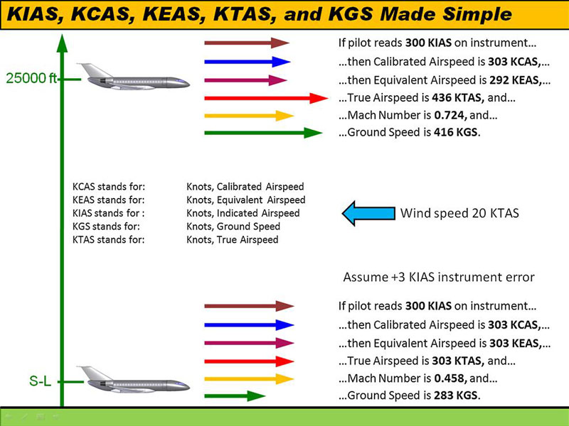
16.3.2 Airspeeds: Instrument, Calibrated, Equivalent, True, and Ground
Instrument Airspeed
This is the airspeed the pilot reads off the airspeed indicator. The reading can be affected by three kinds of error:
(1) Indication error (due to flaws in the instrument itself).
(2) Position error (due to incorrect location of static or pitot sensors).
(3) Pressure lag error (due to rapid change in pressure, such as when a fighter climbs so rapidly the indication system doesn’t keep up with the change in pressure and lags).
When referring to an instrument airspeed using knots as units, it is denoted by the variable VIAS. In the SI system, the units are typically m/s or kmh. In the UK system, the units are ft/s, mph, or knots. It is useful to identify this type of a measurement using the unit KIAS, which stands for knots, indicated airspeed.
Speed of Sound
This is the speed at which pressure propagates through fluid. For air, it can be estimated in terms of ft/s using the following expression:
![]() (16-23)
(16-23)
For altitudes at which GA aircraft are most frequently operated, the ratio of specific heats is 1.4 and the universal gas constant is 1716 ft·lbf/slug·°R, so Equation (16-23) can be simplified as follows:
![]() (16-24)
(16-24)
Calibrated Airspeed
If the error in the airspeed indicator is known, and denoted by the term Δerror, the calibrated airspeed is given by:
![]() (16-25)
(16-25)
For GA aircraft, compliance to 14 CFR Part 23, §23.1587(d)(10), Performance Information, requires a correlation between IAS and CAS to be determined and presented to the operator of the aircraft.
Equivalent Airspeed
The equivalent airspeed is the airspeed the airplane would have to maintain at sea level in order to generate the same compressible dynamic pressure as that experienced at the specific flight condition (altitude and true airspeed). It relates to the true airspeed as follows:
![]() (16-26)
(16-26)
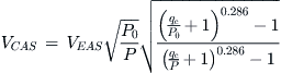
The equivalent airspeed can also be calculated from the calibrated airspeed as follows:
 (16-27)
Note that the power 0.286 is the ratio 1/3.5. It is sometimes useful to convert equivalent airspeed to calibrated airspeed. The following expression can be used for this:
 (16-28)
where the compressible dynamic pressure is given by:
![]() (16-29)
(16-29)
and Mach number:
![]() (16-30)
(16-30)
If the calibrated airspeed is known, the Mach number for compressible flow conditions can be determined from:
![]() (16-31)
(16-31)
where 661.2 is the standard day speed of sound at S-L in knots, VCAS is in KCAS, δ is the pressure ratio, and γ is the specific heat ratio (1.4). Inserting the appropriate values and simplifying allows Equation (16-31) to be written in the following form, which is easier to enter when preparing spreadsheet solutions:
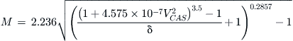 (16-32)
True Airspeed
True airspeed is the airspeed at which the air molecules in the far-field pass the aircraft (since the local molecules accelerate as they pass the airplane). The following expression is used to convert equivalent airspeed to true airspeed:
![]() (16-33)
(16-33)
Ground Speed
Ground speed is the speed at which the aircraft moves along the ground. This speed equals the true airspeed if there is no wind aloft (perfectly calm). However, if windy, the component of the wind parallel to the direction of the aircraft will either add (tailwind) or subtract (headwind) from the true airspeed. If this parallel wind component, denoted by w, is known, then the following expression is used to convert the true airspeed to ground speed:
![]() (16-34)
(16-34)
EXAMPLE 16-4: DETERMINATION OF EAS
Determining EAS may require a sort of inverse process. We would like to be able to look at an airspeed indicator (ASI), read the KIAS and convert it to KEAS. However, instead we have to figure out the KTAS first and then determine what KIAS it corresponds to. It is best to show this process in an example. Determine KTAS, KEAS, and KCAS for an airplane flying at M = 0.45 at 15,000 ft on a standard day.
Solution
Step 1: Compute ambient temperature using Equation (16-14):
![]()
Step 2: Compute speed of sound from Equation (16-23):
![]()
Step 3: Compute true airspeed in ft/s from Equation (16-30):
![]()
Step 4: Compute atmospheric pressure at condition using Equation (16-15):
![]()
Step 5: Compute density at condition using the equation of state:
![]()
Step 6: Compute dynamic pressure, qc, at condition using Equation (16-29):
![]()
Step 7: Compute equivalent airspeed in ft/s at condition using Equation (16-26):
![]()
Step 8: Compute calibrated airspeed in ft/s at condition using Equation (16-28):

Step 9: Convert all airspeeds to knots:
![]()
![]()
![]()
Also, see Figure 16-4 for additional explanations.
16.3.3 Important Airspeeds for Aircraft Design and Operation
The “types” of airspeeds listed in Table 16-4 are of interest to the aircraft designer, from both a performance and certification standpoint. Many can be determined by the analysis methods presented in here. Others are requirements that must be complied with if the aircraft is to be certified.
TABLE 16-4
Important Airspeeds for Aircraft Design and Operation
| V-speed | Description | Article or 14 CFR Part 23 |
| MC | Cruising speed in terms of Mach number. | §23.335 |
| MD | Dive Mach number. | §23.335 |
| MMO | Maximum operating Mach number. | §23.1505 |
| V1 | Maximum speed during take-off at which a pilot can either safely stop the aircraft without leaving the runway or safely continue to V2 take-off even if a critical engine fails (between V1 and V2). | 17.1.3 |
| V2 | Take-off safety speed. Airspeed the airplane must be capable of reaching 35 ft above the ground. | 17.1.2 §23.57 |
| V2min | Minimum take-off safety speed. Minimum value of the V2 airspeed (see V2). Defined for commercial aircraft per 14 CFR 25. | §25.107 |
| V3 | Flap retraction speed. | – |
| VA | Maneuvering speed. A certification airspeed below which the airplane must be capable of full deflection of aerodynamic controls. | 16.4.1 §23.335 |
| VB | Design speed for maximum gust intensity. Most often used for commuter-class aircraft. See Figure 16-13. | §23.335 |
| VBA | Minimum rate-of-descent airspeed, which yields the least altitude lost in a unit time. | 21.3.5 |
| VBG | Best glide speed. Minimum or best angle-of-descent airspeed. This speed will result in the shallowest glide angle and will yield the longest range, should the airplane lose engine power. | 19.2.8 21.3.7 |
| VBR | Airspeed when pilot begins to apply brakes after touch-down. | 22.2.5 |
| VLOF | Lift-off speed. | 17.1.2 |
| Vmax | See VH. | 19.2.10 |
| VMC | Minimum control speed with the critical engine inoperative. | §23.149 |
| VMCA | Minimum control speed while airborne. See VMC. | – |
| VMCG | Minimum control speed on the ground. The minimum airspeed required to counteract an asymmetric yawing moment on the ground due to an engine failure on a multiengine aircraft. | §23.149 |
| VMO | Maximum operating speed. | §23.1505 |
| VMU | Minimum unstick speed. The airspeed at which the airplane no longer “sticks” to the ground. It is a function of the ground attitude (or AOA) of the airplane. The minimum is achieved when the ground attitude is a CLmax or αstall. Defined for commercial aircraft per 14 CFR 25. | §25.107 |
| VNE | Never-exceed speed or maximum structural airspeed. | §23.1505 |
| VNO | Normal operating speed; also called maximum structural cruising speed. It is the speed that should not be exceeded except in smooth air, and then only with caution. | §23.1505 |
| VO | The maximum operating maneuvering speed, VO, is established by the manufacturer as an operating limitation and is not greater than VS √n established in §23.335(c). | §23.1507 |
| VR | Rotation speed. The speed at which the airplane’s nosewheel leaves the ground. It is high enough to ensure the aircraft can reach V2 at 50 ft (GA) or 35 ft (commercial) in the case of an engine failure on a multiengine aircraft. | 17.1.2 §23.51 |
| VREF | Landing reference speed or threshold crossing speed, typically 1.2·VS0 to 1.3·VS0. The factor 1.2 is typically used for military aircraft, but 1.3 for civilian aircraft per §23.73.a | 22.2.5 §23.73 |
| VRmax | Best range speed. The airspeed that results in maximum distance flown. | 19.2.9 |
| VS | Stalling speed or minimum steady flight speed for which the aircraft is still controllable. | 19.2.6 §23.49, §23.335 |
| VS0 | Stalling speed or minimum steady flight speed for which the aircraft is still controllable in the landing configuration. | 19.2.6 §23.49, §23.335 |
| VSR | Reference stalling speed. The stalling speed of the airplane at some condition other than gross weight. Important for heavy aircraft that consume a lot of fuel during a particular mission. The stalling speed at the start of the mission will be higher than at the end. | 19.2.6 22.2.5 |
| VSR0 | Reference stalling speed in landing configuration at some condition other than gross weight. | 19.2.6 22.2.5 |
| VSR1 | Reference stalling speed in a specific configuration at some condition other than gross weight. | 19.2.6 22.2.5 |
| VSW | Speed at which the stall warning will occur. | §23.207 |
| VTD | Touch-down airspeed. | 22.2.5 |
| VTR | Transition airspeed; the average of VLOF and V2. | 17.1.2 |
| VX | The best angle-of-climb airspeed (max altitude gain per unit distance). | 18.3.4 (jet) 18.3.8 (prop) |
| VY | The best rate-of-climb airspeed (max altitude gain per unit time). | 18.3.6 (jet) 18.3.9 (prop) |
| VYSE | The best rate-of-climb airspeed in a multi engine aircraft with one engine inoperative. | 18.3.6 (jet) 18.3.9 (prop) |
aPer 14 CFR Part 23, §23.73 Reference Landing Approach Speed.
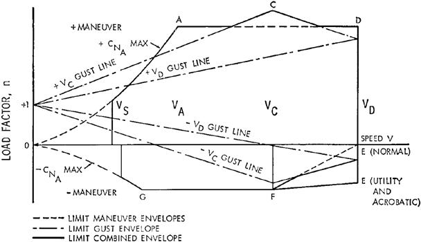
16.4 The Flight Envelope
The purpose of this section is to detail the use of the V-n diagram or flight envelope. The flight envelope shows specific load factors versus airspeed that the airplane has been designed to operate within (see Figure 16-5). It is of primary interest to the structural engineer, but also helps the pilot better understand the limitations of his or her airplane; at what airspeed they can fully deflect control surfaces, what is the dive speed, or the airspeed at which he or she may have to slow down should they encounter turbulent atmospheric conditions, and the list goes on. The V-n diagram is usually prepared in accordance with instructions found in aviation regulations such as 14 CFR Part 23 [6], Part 25 [7], or ASTM F2245 [8], depending on aircraft class. In this section, the construction of a V-n diagram will be shown using 14 CFR Part 23.
Generally, several V-n diagrams are prepared to represent various conditions. Among those are:
(1) Configuration variations (e.g. in T-O, cruise, and landing configuration).
(2) Altitudes (e.g. covering the altitudes from S-L to 20,000 ft and then from 20,000 ft to the design cruise altitude, necessitated by gust loads).
(3) Weight (e.g. empty weight, gross weight, and perhaps some intermediary weights).
An airplane at rest on the ground is acted upon by the force of gravity alone. It is then said to be exerted on by a load factor of 1. If it accelerates for some reason, say upward, because of a force two times larger than its weight, it is said to be subjected to a load factor of 2, and so on. Simply, the load factor is the ratio of the force acting on a body to its unaccelerated weight. A more common expression for this is reacting a 1 g load, a 2 g load, and so on. This is clearly defined in 14 CFR 23.321 General as follows:
Flight load factors represent the ratio of the aerodynamic force component (acting normal to the assumed longitudinal axis of the airplane) to the weight of the airplane. A positive flight load factor is one in which the aerodynamic force acts upward, with respect to the airplane.
The V-n diagram can be thought of as composed of two separate events superimposed on each other to form a complete diagram: maneuvering and gust loading. The aviation regulations always specify how to construct the effect of each event in applicable paragraphs that can be followed almost like instructions in a cookbook. This can be better seen in a moment. To generate a V-n diagram in accordance with 14 CFR 23, follow paragraphs 23.321 through 23.341. The reader not familiar with the regulations is urged to have those handy when following the discussion below for the first time, although the experienced engineers need not. This will be very helpful in understanding the language being used.
In short, the process is as follows: using 14 CFR Part 23, first determine the category the aircraft is to be certified within; i.e. is it a normal, utility, aerobatic, or commuter aircraft? This is imperative as the magnitude of the maneuvering loads depends on this classification. The second step is to gather important and applicable information about the airplane. This includes weight, wing area, lift curve slope, maximum and minimum lift coefficients, to name a few. Then, prepare the maneuvering diagram, followed by the gust diagram. Finally, trace the outline of the diagram. This process is better shown using an example. Remember that all airspeeds used in the V-n diagram are in terms of equivalent airspeed (e.g. KEAS) or Mach number. Here, we will use the former.
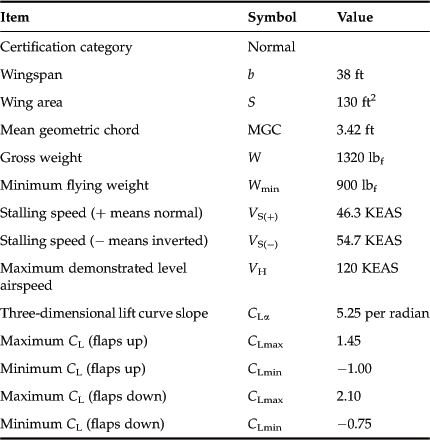
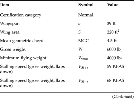
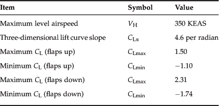
Note that rather than using either of the two sample aircraft to be presented in the next section (the Cirrus SR22 and the Learjet 45XR), a hypothetical aircraft of very light wing loading will be used. This introduces complexity to the generation of the diagram that may perplex even the seasoned aircraft designer. Diagrams for other aircraft are destined to be simpler than the one to be made here and if you can generate the one that follows, you can manage those for the sample aircraft. The sample aircraft for this exercise has the characteristics shown in Table 16-5 and it will be assumed this aircraft is to be certified in the Normal category. Note that it is assumed the aircraft has already been built and flown, as is indicated by the “maximum demonstrated level airspeed” in the table.
16.4.1 Step-by-Step: Maneuvering Loads and Design Airspeeds
This article shows how to step through the regulations to prepare the maneuvering diagram for the above aircraft.
Step 1: Establish Load Factors n+ and n−
Per 14 CFR 23.337(a)(1) estimate the positive load factor that must be used for the aircraft (note that it does not have to be higher than 3.80:
Since n+ > 3.80, we can establish it as 3.80 if we so desire and this is what we will do. Then, 23.337(b)(1) stipulates that the negative load factor, n−, “may not be less than” 0.4 times n+. This clumsily phrased sentence actually means the opposite: n− may not be larger than −0.4·n+; it may be less on the other hand. Of course a lower value presents a limited benefit to the aircraft manufacturer, as this will almost certainly lead to heavier and more expensive to manufacture aircraft. Therefore, n− = −0.4·n+ = −1.52.
Knowing the load factors, we can now calculate the following design airspeeds for the gross weight condition.
Step 2: Design Cruising Speed, VC
The airframe of the airplane must be designed to react gust loads at this airspeed. The purpose is to design the airplane for operation in turbulent air, let alone the possibility of encountering clear air turbulence (CAT), while in cruising flight. The regulations stipulate this must be done assuming a certain minimum value of the cruising speed. Again, the designer can select any speed above (and including) this value, although one must realize the ramifications of selecting a higher cruising speed. The cruising speed should be carefully picked for the following reasons:
(1) Selecting a “certified” cruising speed lower than the cruising speed the airplane is capable of (and at which it will usually be operated) will require the airplane to be slowed down to that speed every time atmospheric turbulence is present. This will irritate even the most docile pilot and may negatively affect the “reputation” of the type in the long run.
(2) Selecting a “certified” cruising speed higher than the cruising speed the airplane is capable of will push up the dive speed (see Step 3) and result in a heavier airframe that has less useful load. Therefore, the proper value of VC should be no higher than the typical and expected cruising speed of the aircraft.
The selection process requires the minimum and maximum cruising speeds to be determined and, then, a representative value between the two to be selected. Per 23.335(a)(1) the minimum cruising speed may not be less than:
Minimum design cruising speed:
![]() (16-36)
(16-36)
Since the wing loading is 1320/130 = 10.2 lbf/ft2 23.335(a)(2) does not apply, but we must check 23.335(a)(3), which says that the cruising speed “need not be more than 0.9·VH.”
Maximum design cruising speed:
![]() (16-37)
(16-37)
For this airplane it is tempting to just go with the upper speed, i.e. VC = 108 KEAS. But first let’s consider what dive speeds these render, assuming it will be 40% greater (as per the regulations, as will be shown shortly). The minimum cruising speed leads to a minimum dive speed of 147.3 KEAS, and the maximum cruising speed requires at least 151 KEAS. However, it might be of interest to ask: why not just select a cruising speed that will result in a dive speed of 150 KEAS? After all, such a number will be easy for the engineering team as well as pilots to remember. It should be stressed that basing the selection of this airspeed on “convenience” is not always the right thing to do, although the author argues it makes sense here. After all, the value is easier to remember than either extreme and guarantees the resulting cruising speed falls between the minimum (105.2 KEAS) and maximum (108 KEAS). It turns out that 150/1.4 = 107 KEAS will result in a VD = 150 KEAS. Therefore, let’s select that as the design cruising speed.
Also, since this is a slow-flying aircraft the stipulations of 23.335(a)(4) does not apply either.
Step 3: Design Dive Speed, VD
This is the maximum airspeed the airplane’s airframe is designed to resist. It is very important as the aircraft must also be free of flutter at airspeed no less than 1.2VD (per 23.629). The dive speed is calculated per 23.335(b)(2) as follows:
However, we decided earlier to design the airplane for 1.40·107 = 150 KEAS and this will comply with the above minimum. This also complies with the previous requirement of 23.335(b)(1). Note that paragraph 23.335(b)(3) does not apply to this aircraft. And paragraph 23.335(b)(4) can be used to reduce the dive speed. However, compliance requires sophisticated analysis and confirmation by flight testing and at this point we will just ignore it and accept the higher dive speed of 150 KEAS.
Step 4: Design Maneuvering Speed, VA
The maneuvering speed is the airspeed below which the aircraft must be capable of withstanding the full deflection of control surfaces.
Maneuvering speed per 23.335(c)(1):
![]() (16-39)
(16-39)
This airspeed is less than VC (107 KEAS) and, therefore, complies with 23.335(c)(2). Also, calculate the negative or inverted maneuvering speed, denoted by G in Figure 16-5. This can be done per Equation (19-8) of Section 19.2.6, Stalling speed, VS, using n = |−1.52| = 1.52, CLmin = |−1.00| = 1.00, and ρ = 0.002378 slugs/ft3.
![]() (16-40)
(16-40)
Step 5: Design Speed for Maximum Gust Intensity, VB
It is best to consider this airspeed after the gust load diagram has been explained. This airspeed is determined in Section 16.4.2, Step-BY-Step: Gust loads.
Step 6: Set Up the Initial Diagram
Having completed determining the above load factors and airspeeds, it is now possible to begin drafting the V-n diagram. This will also help clarify what the above values actually mean. First consider Figure 16-6, which shows a graph with the velocity axis extending from 0 to 160 KEAS and the load factor axis extending from −3 to 5. A number of vertical and horizontal construction lines have been drawn on this graph, but these are used for guidance with the rest of the diagram. The steps taken to accomplish this are labeled as well.
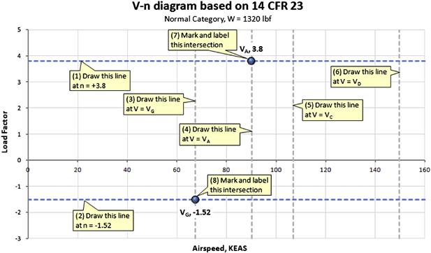
FIGURE 16-6 The first step taken to generate the V-n diagram. The dashed lines are “construction lines” that are removed once the diagram is completed.
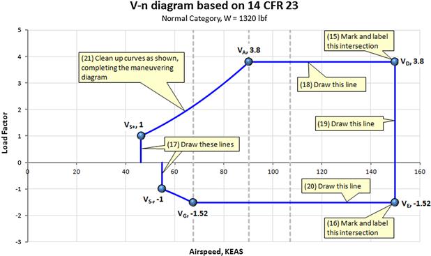
Next perform the following actions illustrated in Figure 16-7. First plot the vertical lines representing the positive and negative stall speeds (see Steps 9 and 10). Next, plot the positive and negative stall lines given by the following expressions:

The constant 0.003388 is simply the product of the S-L density (0.002378 slugs/ft3) and the knots-to-ft/s conversion factor (1.688 – which must be squared due to the term V2), divided by the factor “2” (as in W ≈ L = ½ρV2·S·CLmax). In other words: 0.002378 × 1.6882/2 = 0.003388. The resulting expression conveniently allows the airspeed to be entered in terms of KEAS. With the two curves plotted, the V-n diagram now looks as shown in Figure 16-7. Next create solid lines from the construction lines to represent the outlines of the maneuvering envelope, as shown in Figure 16-8. The next step is to add the gust lines and refine the diagram. This is demonstrated in the next section.
16.4.2 Step-by-Step: Gust Loads
All airplanes are subjected to vertical gusts in level flight. These can be caused by thermals, mountain waves, and other similar atmospheric phenomena. As the airplane penetrates a rising (or sinking) column of air this momentarily changes the angle-of-attack. This either increases (rising column) or decreases (sinking column) the lift of the wing, causing the familiar “bumpiness” to be detected by the occupants as well as the airframe. This is the gust loading. It depends on the forward airspeed of the aircraft and the vertical speed of the rising (or sinking) air penetrated. The aviation authorities specify the gust load requirements in terms of the strength of the vertical speed of the gust.
In magnitude, the gust load ranges from being “annoying” to being so severe it may cause structural failure. For this reason the gust loads must be taken into account when designing the airframe. It must be remembered that the change in AOA does not take place instantaneously, but rather is an event that takes a finite (albeit short) time. Consequently, the resulting gust loads are lessened or “alleviated.” The aviation authorities allow the applicant to reduce the gust load factors by calculating a special gust alleviation factor (see Step 8).
The gust load factors for GA aircraft are determined in accordance with 14 CFR 23.333(c) in accordance with the following rules (see Figure 16-9):
(1) Positive and negative gust velocity of 50 ft/s must be considered at VC at altitudes from S-L to 20,000 ft. Above 20,000 ft, the gust velocity may be reduced linearly to 25 ft/s at 50,000 ft.
(2) Positive and negative gust velocity of 25 ft/s must be considered at VD at altitudes from S-L to 20,000 ft. Above 20,000 ft, the gust velocity may be reduced linearly to 12.5 ft/s at 50,000 ft.
(3) Only applicable to commuter category aircraft, a positive and negative gust velocity of 66 ft/s must be considered at VD at altitudes from S-L to 20,000 ft. Above 20,000 ft, the gust velocity may be reduced linearly to 38 ft/s at 50,000 ft. This gust must be applied at VB.

As stated earlier, the gust load factor is alleviated as calculated in paragraph 23.341(c). This alleviation is based on the assumption that the shape of the gust follows a sinusoidal shape. In other words, the gust gradually rises to the maximum vertical rate as described using the following formula:
![]() (16-43)
(16-43)
where
Ordinarily, this formula is only used to demonstrate the nature of the gust. It is not needed for the actual gust load calculations, which are shown below. The gust load portion of the diagram is created using paragraph 23.341(c). This process requires the gust response to be determined for the four above vertical gust velocities per 23.333(c) (that is ±50 ft/s at VC and ±25 ft/s at VD). For this part, the designer must estimate the lift curve slope for the entire aircraft, although the wing one will usually be sufficient.
It is imperative that the V-n diagram be constructed for all critical configurations, altitudes, and weights. Thus, separate V-n diagrams must be made for the airplane in the clean, take-off, and landing configurations. Making a diagram for the minimum flying weight is equally important to the one at gross weight. While air loads on primary structures like wing spars and skin are greater at gross weight, inertia loads on components that do not directly react aerodynamic loads (e.g. engines, avionics) are higher at minimum weight than at gross weight.
Step 7: Calculated Gust-related Parameters
Start by computing the aircraft mass ratio per 23.341(c) as follows:
![]() (16-44)
(16-44)
where
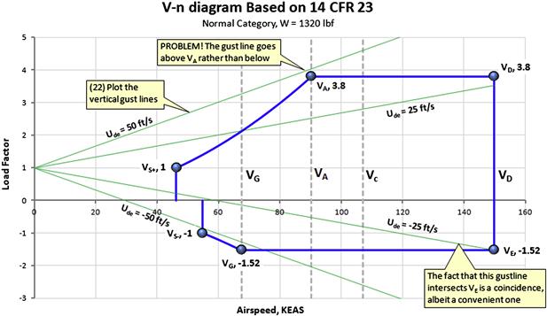
Step 8: Calculate Gust Load Factor as a Function of Airspeed
With the data in Step 7 available, the load factor for each of the four vertical gust velocities (±50 ft/s at VC and ±25 ft/s at VD) can be determined from:
![]() (16-46)
(16-46)
where
Equation (16-46) is used to plot the four gust lines seen in Figure 16-10. The next step is to harmonize the two diagrams and form a single one. Note that a potential issue has surfaced, which is that the positive 50 ft/s gust line goes above VA and not below as shown in Figure 16-5. This will be treated in the next step.
Step 9: Calculate Gust Load Factor as a Function of Airspeed
At this point, it is of interest to determine directly the positive and negative gust load factors. This can be done easily using Equation (16-46):
![]()
Similarly, the negative gust load factor can be found from:
![]()
Step 10: Finalize Gust Diagram
Now, the final presentation of the diagram can be prepared. This is done by identifying all inter sections between the two diagrams, connecting as needed with lines, and resolving any possible trouble areas (see Figure 16-11). It is here that the reason for selecting the particular airplane characteristics becomes apparent. In the author's opinion the diagram in Figure 16-5 is particularly benign in nature. However, the one being created here poses a problem that may seem daunting at first, but it is important to be able to handle it with confidence. The problem is primarily limited to aircraft with low wing loading and is a consequence of the gust lines being too steep.
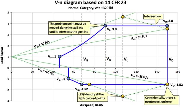
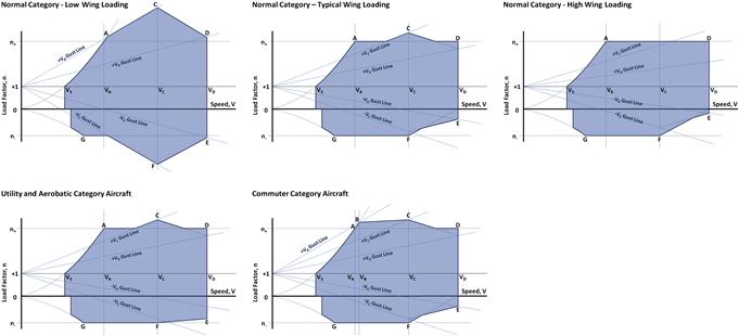
Convenient Relations to Determine Location of Intersections
When plotting the gust load factors it is often necessary to determine the airspeed at which a specific load factor occurs. This is useful when determining the intersection of maneuvering and gust lines. The following expressions can be used for this:
To determine how to extend the positive stall line to the positive 50 ft/s or 66 ft/s gust lines, the load factor calculated per Equation (16-41) must equal that of Equation (16-46). Unfortunately, the expression is more complicated, but the intersection depends on the solution to the following quadratic equation:
![]() (16-49)
(16-49)
Thus, the new VA becomes (ignoring the negative solution):
![]()
Equation (16-49) also conveniently allows the gust penetration speed, VB, to be determined (noting that the vertical gust velocity for the condition is given by Ude = 66 ft/s):
 (16-50)
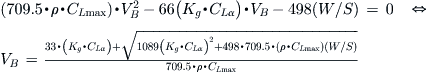
16.4.3 Step-by-Step: Completing the Flight Envelope
The final step in the preparation of the diagram is to combine the maneuvering and gust envelopes. This is shown in Figure 16-12. The shaded region is where the airplane must be demonstrated to operate safely during certification. All the load factors represent limit loads and must be multiplied by a factor of safety of 1.5 to get ultimate loads.
V-n Diagrams with Deployed High-lift Devices
Note that deploying high-lift devices effectively requires a separate envelope to be prepared. This envelope will have its own VA, VD (which is called flap extension speed, denoted by VFE), maneuvering load factor, and so on. The regulatory requirements to establish these values are presented in the appropriate regulations.
The flap is often superimposed on the V-n diagram for a clean configuration.
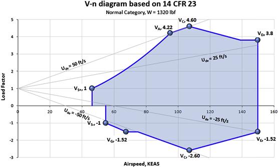
16.4.4 Flight Envelopes for Various GA Aircraft
Although the details of creating a V-n diagram are spelled out in the applicable regulations, not all aspects of this guidance are clear. For this reason, it is easy to become uncertain about the shape of the final diagram. The images in Figure 16-13 provide some guidance as to what shape to expect based on certification category.
IMPORTANT: The V-n diagrams of Figure 16-13 do not reflect the use of high-lift devices.
16.5 Sample Aircraft
The astute aircraft designer is always concerned about the accuracy of calculations. For this reason he or she recognizes the importance of comparing results from the various calculation methods to actual aircraft. A method unable to accurately predict the performance of actual aircraft is limited at best and suspect at worst. The designer must be aware of such limitation, but such knowledge will help him select the right method. This section will introduce two sample aircraft that will be used to demonstrate performance concepts – the Cirrus SR22 and the Learjet 45XR. The former is a piston-powered propeller aircraft and the latter is a twin-engine business jet. Using these aircraft will allow the calculated values to be compared to published data, giving a valuable insight into the accuracy of the methods.
16.5.1 Cirrus SR22
The SR22 (see Figure 16-14) is designed and manufactured by Cirrus Aircraft, of Duluth, Minnesota. The aircraft was conceived as a more powerful derivative of the all-composite SR20, which was designed in the mid 1990s. The SR22 is a four-seat, single-engine, high-performance touring aircraft, and has remained the best-selling aircraft in its class. Powered by a 310 BHP Continental IO-550, six-cylinder horizontally opposed piston engine, it is capable of cruising at 185 KTAS at 75% power at 8000 ft. While boasting high performance, it is designed with safety of operation in mind. The SR20 was the first aircraft in the history of aviation to be certified with an emergency parachute capable of lowering the entire airframe in case of an emergency. By 2013, the parachute system, called Cirrus Airframe Parachute System (CAPS), had saved the lives of some 53 people with 32 deployments [9]. Table 16-6 shows properties of this airplane commonly used in examples in this text. All the data is obtained from the manufacturer’s website (www.cirrusaircraft.com), using published performance data and the analysis methods provided in this book. All geometric data was obtained using the three-view in a manner shown in Figure 16-15. The reader can easily generate data tables of similar nature for all other aircraft using such basics.

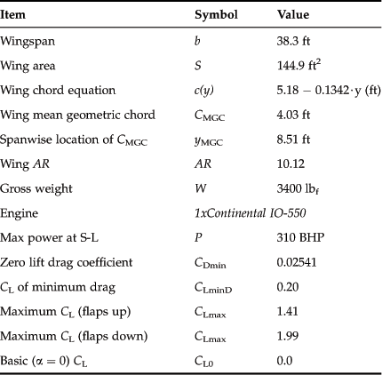
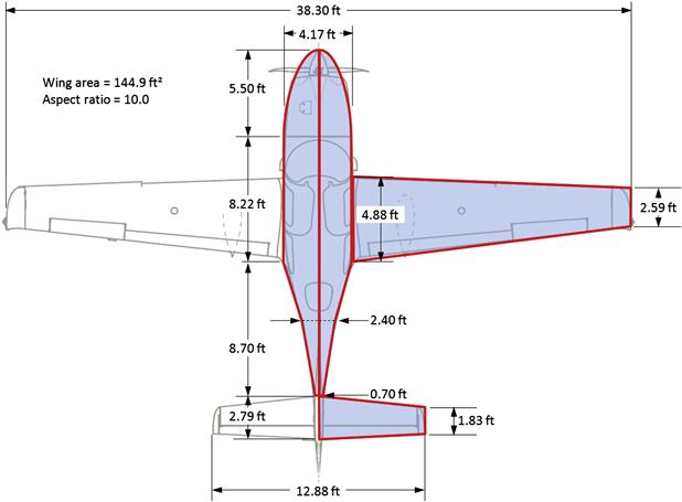
FIGURE 16-15 Scaling the top-view based on the wingspan in the three-view of Figure 16-14 yields the following dimensions. (Courtesy of Cirrus Aircraft)
The reader should be mindful that the data extraction to be implemented for the SR22 can just as well be accomplished for any other type of aircraft. One only needs published geometric, inertia, and performance data, and a proportionally correct three-view drawing. Such data can be obtained from both the type certificate data sheet (TCDS [10]) and the Pilots Operation Handbook (POH), both of which are readily available; the former from the FAA website (www.faa.gov) and the latter from pilots. Be careful, however: POH data is copyrighted and cannot be made public in the manner shown here. Cirrus Aircraft has graciously given permission for the presentation of the data extracted in this text and this is fortunate, because the SR22 has far more exciting performance and handling characteristics than most aircraft in its class and, thus, offers great learning potential on how to design fast and efficient single-engine aircraft.
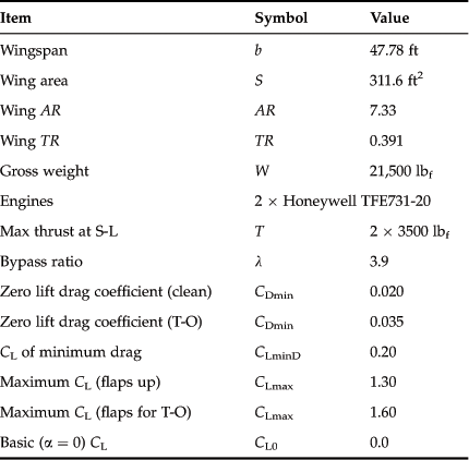
16.5.2 Learjet 45XR
Jet performance concepts will be demonstrated using the Learjet 45XR business jet (see Figure 16-16). Learjet was founded by an American inventor and a very original and influential business man, William P. Lear (1902–1978). Learjet produced a number of well-known business jets, such as the original Learjet 23, the first in a family of high-performance aircraft. In 1969, Learjet merged with Gates Aviation, forming Gates Learjet Corporation, and in 1990 the company was acquired by Bombardier Aerospace. The development of the 45XR was announced by Bombardier in September 1992 and the first flight of the prototype aircraft took place on October 7, 1995. FAA certification was granted in September 1997. The aircraft is powered by two FADEC-controlled Honeywell TFE731-20 engines and is equipped with an internal auxiliary power unit (APU) for ground power. The Learjet 45XR is a special version of the Learjet 45 and was introduced in June 2004. The 45XR offers higher take-off weight, faster cruising speeds and faster rate-of-climb than its predecessor, thanks to a more powerful engine. Simplified and “assumed” values for the 45XR are presented in Table 16-7.

Exercises
(1) Determine the pressure, temperature and density and the corresponding ratios for the following conditions:
(a) Altitude of 10,000 ft for outside air temperature (OAT) differing some −30 °F, 0 °F, and 30 °F from the ISA temperature (ISA is the 0 °F condition).
(b) Altitude of 8.4 km for OAT differing some −30 °C, 0 °C, and 30 °C from the ISA temperature.
(2) Convert the following airspeeds into ft/s:
(g) The average of 121 mph, 65 knots, and 110 kmh
(3) Convert the following airspeeds into knots:
(g) The average of 32 mph, 48 m/s, and 62 kmh
(4) Determine the KTAS for the following airspeeds and altitudes (all airspeeds are calibrated airspeeds. Ignore compressibility):
(a) 150 m/s at an altitude of 10,550 m
(b) 276 kmh at an altitude of 3.3 statute miles
(c) 432 ft/s at an altitude of 7.6 km
(d) 299 mph at an altitude of 5.6 nm
(5) Determine the KTAS for the following airspeeds and altitudes and OATs (ignore compressibility):
(a) 225 KCAS at an altitude of 6000 ft at ISA
(b) 145 KIAS at an altitude of 15,000 ft at ISA+20 °C. Instrument error is −3 KIAS
(c) 270 KIAS at an altitude of 35,000 ft at ISA−20 °C. Instrument error is +1.2%
(6) Determine the KIAS for the following airspeeds and altitudes and OATs (ignore compressibility):
(a) 225 KTAS at an altitude of 6000 ft at ISA
(b) 145 KTAS at an altitude of 15,000 ft at ISA+20°C. Instrument error is −3 KIAS
(c) 270 KTAS at an altitude of 35,000 ft at ISA−20°C. Instrument error is +1.2%
(7) Determine the KGS for the following airspeeds and altitudes and OATs and wind speeds (ignore compressibility):
(a) 225 KTAS at an altitude of 6000 ft at ISA. Headwind is 35 knots
(b) 227 KIAS at an altitude of 15,000 ft at ISA+15°C. Instrument error is +2.5 KIAS. Headwind is −18 knots
(c) 270 KIAS at an altitude of 35,000 ft at ISA-30°C. Instrument error is +2.8%. Headwind is −95 knots
(8) Determine KTAS, KEAS, and KCAS for an airplane flying at M = 0.8 at 36,000 ft on a standard day. If the instrument error is −3.5 KIAS, determine the indicated airspeed as well.
(9) Create a V-n diagram for the aircraft presented in the table below.
Variables
| Symbol | Description | Units (UK and SI) |
| a | Lapse rate | |
| a | Speed of sound | |
| a0 | Speed of sound at S-L on a standard day | |
| AR | Aspect ratio | |
| b | Wingspan | ft or m |
| c(y) | Function for determining wing chord at specified span location | ft or m |
| CL0 | Lift coefficient at zero AOA | |
| CLmax | Maximum lift coefficient | |
| CLmin | Minimum lift coefficient | |
| CLminD | Lift coefficient at minimum drag | |
| CLα | 3D lift curve slope | /degree or /radian |
| h | Altitude | ft or m |
| h0 | Reference altitude | ft or m |
| hP | Pressure altitude | ft or m |
| hρ | Density altitude | ft or m |
| k | Lapse rate constant | |
| Kg | Gust alleviation factor | |
| MC | Cruising Mach number | |
| MD | Diving Mach number | |
| MGC | Mean geometric chord | ft or m |
| MMO | Maximum operating Mach number | |
| n− | Negative load factor | |
| n+ | Positive load factor | |
| ng | Gust load factor | |
| p | Pressure | lbf/ft2 or Pa |
| P | Maximum power at S-L | ft·lbf/s or N·m/s |
| p0 | Reference S-L pressure | lbf/ft2 or Pa |
| pmbar | Pressure in mbar | mbar |
| pPa | Pressure in Pa | Pa |
| ppsf | Pressure in psf | lbf/ft2 |
| ppsi | Pressure in psi | lbf/in2 |
| qc | Compressible dynamic pressure | lbf/ft2 or Pa |
| R | Specific gas constant for air | ft·lbf/(slug·°R) or m2/(K·s) |
| Re | Reynolds number | |
| RH | Relative humidity | |
| RH2O | Specific gas constant for water vapor | ft·lbf/(slug·°R) or m2/(K·s) |
| S | Wing area | ft2 or m2 |
| T | Temperature | °R or K |
| T°C | Temperature in degrees Celsius | °C |
| T°F | Temperature in degrees Fahrenheit | °F |
| T°R | Temperature in degrees Rankine | °R |
| T0 | Temperature at reference altitude | °R or K |
| TK | Temperature in degrees Kelvin | K |
| TR | Taper ratio | |
| U | Maximum vertical gust rate | |
| Ude | Vertical gust velocity | ft/s or m/s |
| V1 | Maximum speed at which a multiengine aircraft can be stopped if critical engine fails during take-off | Knots (typ.) or ft/s or m/s |
| V2 | Take-off safety speed | Knots (typ.) or ft/s or m/s |
| V2min | Minimum take-off safety speed | Knots (typ.) or ft/s or m/s |
| V3 | Flap retraction speed | Knots (typ.) or ft/s or m/s |
| VA | Maneuvering speed | Knots (typ.) or ft/s or m/s |
| VB | Design speed for maximum gust intensity | Knots (typ.) or ft/s or m/s |
| VBA | Minimum rate-of-descent airspeed | Knots (typ.) or ft/s or m/s |
| VBG | Best glide speed | Knots (typ.) or ft/s or m/s |
| VBR | Airspeed when pilot begins to apply brakes after touch-down | Knots (typ.) or ft/s or m/s |
| VC | Design cruising speed or maximum structural speed | Knots (typ.) or ft/s or m/s |
| VC55% | Cruising speed at 55% power | Knots (typ.) or ft/s or m/s |
| VC65% | Cruising speed at 65% power | Knots (typ.) or ft/s or m/s |
| VC75% | Cruising speed at 75% power | Knots (typ.) or ft/s or m/s |
| VCAS | Calibrated airspeed | Knots (typ.) or ft/s or m/s |
| VCmax | Maximum cruising speed | Knots (typ.) or ft/s or m/s |
| VCmin | Minimum design cruising speed | Knots (typ.) or ft/s or m/s |
| VD | Dive speed | Knots (typ.) or ft/s or m/s |
| VEAS | Equivalent airspeed | Knots (typ.) or ft/s or m/s |
| VEF | Speed at which critical engine is assumed to fail during take-off | Knots (typ.) or ft/s or m/s |
| VEmax | Best endurance speed | Knots (typ.) or ft/s or m/s |
| VF | Design cruising speed for negative load factor | Knots (typ.) or ft/s or m/s |
| VFE | Maximum flap extension speed | Knots (typ.) or ft/s or m/s |
| VFLR | Airspeed for initiating flare maneuver | Knots (typ.) or ft/s or m/s |
| VFTO | Final take-off speed | Knots (typ.) or ft/s or m/s |
| VG | Negative maneuver speed | Knots (typ.) or ft/s or m/s |
| VGS | Ground speed | Knots (typ.) or ft/s or m/s |
| VIAS | Indicated airspeed | Knots (typ.) or ft/s or m/s |
| VLDmax | Best glide speed | Knots (typ.) or ft/s or m/s |
| VLE | Maximum landing gear extended speed | Knots (typ.) or ft/s or m/s |
| VLO | Maximum landing gear operating speed | Knots (typ.) or ft/s or m/s |
| VLOF | Lift-off speed | Knots (typ.) or ft/s or m/s |
| Vmax | Maximum obtainable level airspeed | Knots (typ.) or ft/s or m/s |
| VMC | Minimum control speed with critical engine inoperative | Knots (typ.) or ft/s or m/s |
| VMCA | Minimum control speed while airborne | Knots (typ.) or ft/s or m/s |
| VMCG | Minimum control speed on the ground | Knots (typ.) or ft/s or m/s |
| VMO | Maximum operating speed | Knots (typ.) or ft/s or m/s |
| VMU | Minimum unstuck speed | Knots (typ.) or ft/s or m/s |
| VNE | Never-exceed speed | Knots (typ.) or ft/s or m/s |
| VNO | Normal operating speed | Knots (typ.) or ft/s or m/s |
| VO | Maximum operating maneuvering speed | Knots (typ.) or ft/s or m/s |
| VR | Rotation speed | Knots (typ.) or ft/s or m/s |
| VREF | Landing reference speed | Knots (typ.) or ft/s or m/s |
| VRmax | Speed of best range | Knots (typ.) or ft/s or m/s |
| VS0 | Stall speed flaps down | Knots (typ.) or ft/s or m/s |
| VS1 | Stall speed clean | Knots (typ.) or ft/s or m/s |
| VSR | Reference stalling speed | Knots (typ.) or ft/s or m/s |
| VSR0 | Reference stalling speed in landing configuration | Knots (typ.) or ft/s or m/s |
| VSW | Speed at which stall warning occurs | Knots (typ.) or ft/s or m/s |
| VTAS | True airspeed | Knots (typ.) or ft/s or m/s |
| VTD | Touch-down speed | Knots (typ.) or ft/s or m/s |
| VTR | Transition airspeed | Knots (typ.) or ft/s or m/s |
| VX | Best angle-of-climb airspeed | Knots (typ.) or ft/s or m/s |
| VY | Best rate-of-climb airspeed | Knots (typ.) or ft/s or m/s |
| VYSE | OEI best rate-of-climb | Knots (typ.) or ft/s or m/s |
| W | Gross weight | lbf or N |
| W0 | Gross weight | lbf or N |
| Wmin | Minimum flying weight | lbf or N |
| x | Humidity ratio (context dependent) | ft or m |
| x | distance penetrated into gust (context dependent) | ft or m |
| Δerror | Error in airspeed indicator | ft/s or m/s |
| ΔTISA | Deviation from International Standard Atmosphere | °R or K |
| δ | Pressure ratio | |
| γ | Specific heat ratio | |
| λ | Bypass ratio | |
| μ | Viscosity | lbf·s/ft2 or N·s/m2 |
| μg | Aircraft mass ratio | |
| ν | Kinematic viscosity | 1/(ft2·s) or 1/(m2·s) |
| θ | Temperature ratio | |
| ρ | Density | slugs/ft3 or kg/m3 |
| ρ0 | Reference S-L density | slugs/ft3 or kg/m3 |
| ρkg/m3 | Density in kg/m3 | kg/m3 |
| ρS-L | Density at sea level | |
| ρslugs/ft3 | Density in slugs/ft3 | slugs/ft3 |
| ρstd | Density at altitude, calculated by standard methods | slugs/ft3 or kg/m3 |
| σ | Density ratio |
References
1. http://www.fai.org/records/powered-aeroplanes-records.
2. http://www.nasa.gov/centers/dryden/history/pastprojects/Helios/index.html.
3. http://www.nasa.gov/pdf/64317main_helios.pdf.
4. http://www.uwsp.edu/geo/faculty/ritter/geog101/textbook/atmospheric_moisture/lapse_rates_1.html.
5. http://www.vaisala.com/humiditycalculator/help/index.html#calculating-humidity.
6. Code of Federal Regulations, 14 CFR Part 23.
7. Code of Federal Regulations, 14 CFR Part 25.
8. ASTM International, formerly known as the American Society for Testing and Materials.
9. http://www.cirruspilots.org/Content/CAPSHistory.aspx.
10. TCDS A00009CH, Cirrus Design Corporation, Revision 18, 12/29/2011, FAA.