
Performance – Take-Off
Abstract
The chapter presents T-O performance methods. First, fundamental relations of the T-O ground run, including the equation of motion for a T-O ground run and the kinematics of the T-O run are presented. Then, several methods to solve the equation of motion are introduced. These include standard, but limited solutions and a very capable numerical method that allows the introduction of time dependent events to be taken into account. These could be a time dependent increase in flap deflection or power increase. Finally, the T-O characteristics of selected aircraft types are presented to allow the reader an accessible reference to actual aircraft data.
Keywords
Equation of motion; free-body; ground roll; rotation; transition; climb; balanced field length; take-off; acceleration; brake-release; asphalt; turf; wet grass; numerical integration method; tricycle; taildragger; sensitivity
Outline
17.1.1 The Content of this Chapter
17.1.2 Important Segments of the T-O Phase
17.1.3 Definition of a Balanced Field Length
17.2 Fundamental Relations for the Take-off Run
17.2.1 General Free-body Diagram of the T-O Ground Run
17.2.2 The Equation of Motion for a T-O Ground Run
Derivation of Equations (17-4) and (17-5)
17.2.4 Formulation of Required Aerodynamic Forces
17.2.5 Ground Roll Friction Coefficients
17.2.6 Determination of the Lift-off Speed
Requirements for T-O Speeds Per 14 CFR Part 23 for GA Aircraft
Requirements for T-O Speeds Per 14 CFR Part 25 for Commercial Aviation Aircraft
17.2.7 Determination of Time to Lift-off
17.3 Solving the Equation of Motion of the T-O
17.3.1 Method 1: General Solution of the Equation of Motion
Step 2: Lift-induced Drag in Ground Effect
Step 3: Lift at the Reduced Lift-off Speed
Step 4: Drag at the Reduced Lift-off Speed
Step 5: Thrust at the Reduced Lift-off Speed
17.3.2 Method 2: Rapid T-O Distance Estimation for a Piston-powered Airplane
Derivation of Equation (17-21)
17.3.3 Method 3: Solution Using Numerical Integration Method
Propeller Thrust at Low Airspeeds
17.3.4 Determination of Distance During Rotation
17.3.5 Determination of Distance for Transition
Derivation of Equations (17-26) and (17-27)
17.3.6 Determination of Distance for Climb Over an Obstacle
17.3.7 Treatment of T-O Run for a Taildragger
17.3.8 Take-off Sensitivity Studies
17.1 Introduction
It is appropriate to start the performance analysis with one of the most important maneuvers performed by any aircraft; the take-off (T-O). Figure 17-1 shows an organizational map displaying the T-O among other parts of the performance theory. It is of utmost importance that the designer not only understands the T-O capabilities of the new design, but also recognizes its limitations and sensitivity. This chapter will present the formulation of and the solution of the equation of motion for the entire T-O maneuver and present practical as well as numerical solution methodologies that can be used both for propeller- and jet-powered aircraft.
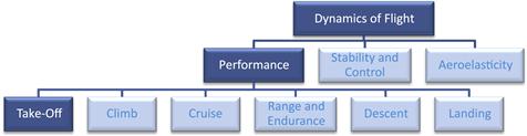
FIGURE 17-1 An organizational map placing performance theory among the disciplines of dynamics of flight, and highlighting the focus of this section; T-O performance analysis.
T-O performance typically refers to the distance required for the aircraft to accelerate from a standstill to lift-off, as well as the distance required to attain an initial and steady climb. Most aircraft are designed to meet specific runway length requirements, and these may dictate the power plant necessary, as most aircraft use far less power for cruise than for the T-O and climb. As an example of the constraints confronting the designer, commercial aircraft must be at least capable of operating from runways used by the competition, and preferably from even shorter runways, as this might expand their marketability and give them a competitive edge.
Aircraft are sometimes required to meet some T-O distance requirements specified in a request for proposal (RFP) or specific design requirements. In order to meet such requirements the designer must not only consider the T-O distance at ISA and S-L, but also runways that present the design with an uphill slope, as well as on a hot day and high-altitude conditions. All can seriously tax the capability of the aircraft. There may even be a combination of high temperatures in locations at high elevation. These are altogether easy to overlook. As an example, the Mariscal Sucre International Airport in Quito, Ecuador, is at an altitude of 9228 ft and presents a serious high-altitude challenge to commercial aircraft. The largest type of aircraft to regularly operate from it is the Airbus A-340.
In order to evaluate the capability of the aircraft the designer should prepare a T-O sensitivity graph, which shows the T-O run as a function of density altitude and shows the impact of a selected parameter, e.g. weight or outside air temperature, on the operation of the aircraft. A typical such graph is shown in Section 17.3.8, Take-off sensitivity studies. Preparing the analysis in a spreadsheet is very convenient and a considerable amount of information about the airplane’s capabilities can be learned from such a tool.
A capable T-O performance analysis also accounts for the type of landing gear featured on the aircraft. The analysis in this text assumes conventional tricycle or taildragger configurations. Accounting for landing gear is particularly important for taildraggers. A taildragger lifts the tailwheel off the runway as soon as certain airspeed is achieved. The airspeed at which this takes place may range from standstill to half of the airplane’s lift-off speed. However, as soon as this happens, the T-O formulation must be modified to account for two rather than three landing gear contact points and the associated reduction in drag of the more horizontal configuration. This is discussed further in Section 17.3.7, Treatment of T-O run for a taildragger.
In general, the methods presented here are the industry standard and mirror those presented by a variety of authors, e.g. Perkins and Hage [1], Torenbeek [2], Nicolai [3], Roskam [4], Hale [5], Anderson [6] and many, many others.
17.1.1 The Content of this Chapter
• Section 17.2 presents the fundamental relations of the T-O ground run, including the equation of motion for a T-O ground run and the kinematics of the T-O run.
• Section 17.3 presents several methods to solve the equation of motion.
• Section 17.4 presents the T-O properties of selected aircraft types.
17.1.2 Important Segments of the T-O Phase
Generally, the T-O phase is split into the segments shown in Figure 17-2. The ground roll is the distance from brake release to the initiation of the rotation, when the pilot pulls the control wheel (or stick or yoke) backward in order to raise the nose of the aircraft. This maneuver is required to increase the AOA of the airplane to help it become airborne. The aircraft typically remains in this attitude for some 1–3 seconds, depending on aircraft size, before the tires lose contact with the ground. This segment is called the rotation. The rotation phase concludes as the aircraft lifts off the ground and begins the transition and subsequent climb phase.

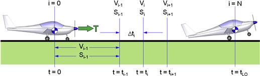
In short, the purpose of the T-O analysis is to estimate the total T-O distance by breaking it up into the aforementioned segments and analyzing each step using simplified physics. Typically, requirements for aircraft design call for the ground roll and the total T-O distance to be specified. The first step prior to formulating the problem is to define the segments using variable denotation that will be carried through the remainder of this section. This is shown in Figure 17-3.
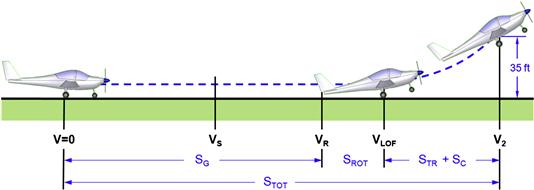
The airspeeds referenced in Figure 17-3 used in the T-O analysis are shown in Table 17-1.
TABLE 17-1
Definition of Important Airspeeds for the T-O
| Name | Airspeed | GA Aircraft (FAR 23)a |
| Ground run | VR | 1.1VS1 |
| Rotation | VLOF | 1.1VS1 |
| Transition | VTR | 1.15VS1 |
| Climb | V2 | 1.2VS1 |
aAirspeeds are formally established per 14 CFR Part 23, § 23.51 Takeoff Speeds.
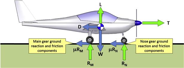
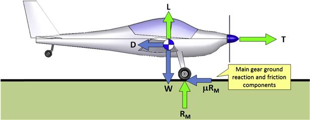
The nature of the formulation of the T-O segments depends in part on the airplane’s landing gear. To better understand why, consider Figure 17-4, which shows the T-O maneuver for two of the most common landing gear configurations: a tricycle and a taildragger.
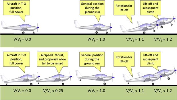
In Figure 17-4, V is the instantaneous airspeed of the aircraft and VS is the stalling speed in the T-O configuration. This means that if the airplane features high-lift devices, VS refers to the stalling speed with flaps deployed. The important point is that the airplane must accelerate from standstill to a given airspeed, called the lift-off speed, before it can, well, lift off. The tricycle configuration accelerates with the main and nose landing gears in contact with the ground. However, the taildragger, initially, has the main landing gear and tailwheel in contact with the ground until a combination of forward airspeed, thrust, and propwash over the horizontal tail allows it to lift the tailwheel off the ground. For some taildraggers, typically light ones, this happens as soon as the engine generates T-O thrust. For others, primarily larger aircraft, some forward airspeed must be acquired before the tail can be raised off the ground. Sections 13.3.4, Tricycle landing gear reaction loads and 13.3.5, Taildragger landing gear reaction loads, provide methods to estimate the airspeed at which a tricycle configuration can lift the nose gear off the ground and at which a taildragger can lift the tailwheel off the ground.
A T-O analysis of a tricycle and taildragger aircraft differs primarily in having to account for the tail of the latter being raised off the ground. Initially, the taildragger geometry is one of an airplane at a high AOA, whereas once the tailwheel is off the ground it transforms into one at a low AOA. A proper representation of the transformation is required for accurate estimation of the T-O for such airplanes.
The distance covered in the specific segments shown in Figure 17-3 are determined in the sections shown in Table 17-2.
TABLE 17-2
Sections Used to Estimate Various Segments of the T-O Run
| Segment Name | Symbol | Section |
| Ground roll | SG | 17.3.1 through 17.3.3 |
| Rotation | SR | 17.3.4 Determination of distance during rotation |
| Transition | STR | 17.3.5 Determination of distance for transition |
| Climb | SC | 17.3.6 Determination of distance for climb over an obstacle |
A schematic of the T-O run showing other important airspeeds is shown in Figure 17-5. See Table 16-4 for the definition of the various airspeeds. It should be made clear that the stalling speed (VS) must be exceeded before the airplane can become airborne, and that it is always based on the configuration of the aircraft during the T-O run. Thus, if the airplane takes off with its flaps deflected (typical deflection is somewhere between 10° and 20°) its stalling speed will be less than in the clean configuration. The minimum control speed with one engine inoperative (VMC) only applies to multiengine aircraft.

The unstick speed is the airspeed at which the airplane no longer ‘sticks’ to the runway and lifts off whether one wants it to or not. It depends on the attitude (or AOA) of the airplane during the ground run. It is high if the ground run attitude is low and reduces as the attitude is increased (in other words: the higher the nose, the lower the unstick speed). It follows that the minimum unstick speed (VMU) is achieved when the airplane is in a tail-strike position (at its maximum rotation angle). Clearly, VMU is will be lower than the lift-off speed (VLOF), as the airplane is only rotated to its maximum rotation angle due to pilot error (which may be compounded by very aft CG).
17.1.3 Definition of a Balanced Field Length
Consider Figure 17-6, which shows how the airspeed of a typical aircraft changes with respect to distance from brake release during a T-O run. Assume this graph reflects the relationship between airspeed and runway distance of a multiengine aircraft. Initially, while at stand-still, the airspeed and runway distance are both zero. However, as soon as the pilot increases thrust and releases the brakes, the aircraft begins to accelerate and the distance from brake release increases.

Now, assume that some distance from brake release one engine becomes inoperative. The airplane will continue to accelerate, only much slower than before. Now two things can happen:
(1) If the airspeed is low (and the distance covered is short), the pilot can simply step on the brakes and bring the aircraft to a complete stop before running out of runway. Problem solved. This is shown in the left-hand graph in Figure 17-7.

FIGURE 17-7 If the failure occurs early enough it is possible to stop the airplane in time (left). However, if it is moving too fast it may not be able to stop in time, but may still be able to lift-off before running out of runway (right).
(2) On the other hand, if the airspeed is high (assuming the airplane is still on the ground) there may not be enough runway ahead of the plane to fully stop it in time, so braking is not an option. In this case, two new things can happen:
(a) There is insufficient thrust remaining to accelerate to lift-off before running out of runway. Disaster strikes. (The pilot should never have attempted the T-O run.)
(b) There is indeed enough thrust remaining to accelerate to lift-off before running out of runway. Disaster is avoided. This is shown in the right-hand graph in Figure 17-7.
While this logic is sound it requires analysis effort which may not be possible in a time of crisis. Also note that the following can be deduced from the graphs in Figure 17-7. If there is an airspeed at which the airplane can be stopped in time (as shown in the left graph) and there is an airspeed at which it cannot be stopped in time, but accelerated to lift-off (as shown in the right graph), then there must be an airspeed between the two at which it can both be stopped and accelerated to lift-off in time (if not, then the runway is too short for a safe operation of the airplane). There is indeed such an airspeed and it has been given a special name: V1.
In order to avoid exerting analysis effort in a time of crisis and, that way, increase safety, it is simpler to tell the pilot that if below V1, step on the brakes; and if above, continue the take-off. The distance required to accelerate the aircraft to V1 and then decelerate it to a complete stop by applying hard braking, is also given a special name; balanced field length (sometimes called accelerate-stop distance). Strictly speaking it is only applicable to multiengine airplanes, since a single-engine airplane has no choice but to apply the brakes. The importance of the BFL is that it gives the pilot two safe options.
Torenbeek [2, pp. 168–169] developed the following empirical expression to estimate the balanced field length for a multiengine aircraft, presented here using the original symbols:
![]() (17-1)
(17-1)
where
CL2 = magnitude of the lift coefficient at V2. If V2 = 1.2VS, then it can be shown that CL2 = 0.694CLmax
g = acceleration due to gravity = 32.174 ft/s2 or 9.807 m/s2
hto = obstacle height = 35 ft (10.7 m) for commercial jetliners and 50 ft (15.2 m) for GA aircraft
S = reference wing area, ft2 or m2
Wto = take-off weight, lbf or N
![]() average thrust during the T-O run, given by Equations (17-2) and (17-3).
average thrust during the T-O run, given by Equations (17-2) and (17-3).
ρ = air density, in slugs/ft3 or kg/m3
μ′ = 0.01·CLmax + 0.02, where CLmax is that of the T-O configuration

Torenbeek’s method requires the average thrust during the T-O run to be estimated for jets and propeller-powered aircraft using the following expressions:
![]() (17-2)
(17-2)
where
Tto = maximum static thrust, in lbf or N
For an aircraft with a constant-speed propeller:
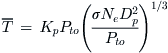 (17-3)
where
Dp = propeller diameter, in ft or m
Pto = maximum engine power, in BHP or kg·m/s (which is power in watts divided by g)
![]()
Note that for a fixed-pitch propeller, the average thrust will be approximately 15–20% lower than that for the constant-speed propeller.
EXAMPLE 17-1
Estimate the balanced field length for the Learjet 45XR assuming a maximum lift coefficient in the T-O configuration to be 1.60 and V2 = 1.2VS. Also, assume an obstacle height of 50 ft and gross weight of 21,500 lbf. Note that other properties of the airplane are given in Table 16-7. Assume the simplified drag model and that the Oswald span efficiency factor amounts to 0.8294 and CDmin = 0.035 in the T-O configuration. Furthermore, assume the maximum thrust with one engine inoperable (OEI) to equal one half of the average thrust calculated in Step 4 below.
Solution
Step 1: Determine the constant “k”:
![]()
Step 2: Calculate the stalling speed in the T-O configuration using the given CLmax and Equation (19-7):
![]()
Step 3: Therefore, V2 amounts to:
![]()
Step 4: Calculate the average thrust during the T-O run, ![]() , using Equation (17-2):
, using Equation (17-2):
![]()
Step 5: Determine the factor μ′: μ′ = 0.01·CLmax + 0.02 = 0.036.
Step 6: Estimate the drag at the airspeed V2. Note that this requires the drag polar for the aircraft to be known. Here, assume the following drag polar for the aircraft in the T-O configuration: CD = CDmin + k·CL2 = 0.035 + 0.05236 CL2.
Step 7: Estimate climb angle at V2 and the difference Δγ2. As stated in the introduction to this example, it will be assumed that the thrust with OEI amounts to one half that of ![]() calculated in Step 4, or 2955 lbf. This yields the following climb angle:
calculated in Step 4, or 2955 lbf. This yields the following climb angle:
![]()
Step 8: Finally calculate the BFL using Equation (17-1):

This compares to 5040 ft published by Ref. [7] for the type.
17.2 Fundamental Relations for the Take-off Run
In this section, the equation of motion for the T-O will be derived, as well as some elementary relationships that can be used to evaluate the ground run segment of the T-O maneuver. Both conventional and taildragger configurations will be considered.
17.2.1 General Free-body Diagram of the T-O Ground Run
Figure 17-8 and Figure 17-9 show the free-body diagrams of tricycle and taildragger configurations during a developed T-O ground run.
17.2.2 The Equation of Motion for a T-O Ground Run
The equation of motion for an aircraft during the ground run on a perfectly horizontal and flat runway can be estimated from:
Acceleration on a flat runway:
![]() (17-4)
(17-4)
where
D = drag as a function of V, in lbf or N
g = acceleration due to gravity, ft/s2 or m/s2
L = lift as a function of V, in lbf or N
W = weight, assumed constant in lbf or N
μ = ground friction coefficient (see Table 17-3)
If the runway is not perfectly horizontal, but has an uphill or downhill slope γ (see Figure 17-10), the acceleration of the aircraft should be estimated from:
Acceleration on an uphill slope γ:
![]() (17-5)
(17-5)
where γ = slope of runway (if uphill the sign is positive but negative if downhill), in °.

FIGURE 17-10 A balanced 2D free-body (forces only) of the T-O ground run for a tricycle gear aircraft on an uphill slope runway.
Note that Equation (17-5) assumes the reference frame to be aligned along the runway. This is a reasonable assumption because the runway length reported will be along the slope. We can also rewrite this to get the acceleration in terms of the thrust-to-weight ratios:
![]() (17-6)
(17-6)
Derivation of Equations (17-4) and (17-5)
Consider the aircraft in Figure 17-8 and Figure 17-9. Its motion can be completely described using the standard equations of motion as follows. First, the sum of the forces in the x-direction must equal the airplane’s horizontal acceleration:
![]() (i)
(i)
where μ is the coefficient of friction caused by a ground friction. Its value depends on the runway surface. Suitable values can be seen in Table 17-3. Additionally, the forces in the y-direction must yield no net vertical acceleration:
![]()
Solving for the horizontal acceleration dV/dt results in:
![]()
The resulting expression is shown as Equation (17-4). Note that if the aircraft is accelerating along an uphill or downhill runway, whose slope is given by γ, then Equation (i) must include an additional component caused by its weight:
![]() (ii)
(ii)
The resulting expression is shown as Equation (17-5). If the runway is uphill, the sign for γ should be positive, as this will cause the resulting acceleration to be less than on a perfectly horizontal runway. Likewise, if the runway is downhill, the sign for γ should be negative, as this will cause the resulting acceleration to be higher than on a perfectly horizontal runway.
QED
17.2.3 Review of Kinematics
Kinematics is the study of the motion of objects that only involves the motion itself (e.g. acceleration, speed, and distance) and not what causes it (forces and moments). The kinematic formulation is essential for the study of the take-off run. The most basic formulation is presented below:
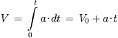 (17-7)
 (17-8)
Alternative expression for distance:
![]() (17-9)
(17-9)
EXAMPLE 17-2
The pilot’s operating handbook (POH) for the single engine, four-seat, SR22 gives a lift-off speed of 73 KCAS and T-O distance of 1020 ft (ISA at S-L). Estimate the average acceleration and time in seconds from brake release to lift-off.
17.2.4 Formulation of Required Aerodynamic Forces
In this section, the following formulation of aerodynamic forces is assumed when considering the T-O maneuver.
![]() (17-10)
(17-10)
![]() (17-11)
(17-11)
![]() (17-12)
(17-12)
![]() (17-13)
(17-13)
![]() (17-14)
(17-14)
![]() (17-15)
(17-15)
where
CDi(CL TO) = induced drag coefficient of aircraft during the T-O run
Note that the induced drag must be corrected for ground effect, in particular if the airplane uses flaps or if its attitude is such that its ground run AOA is high. Refer to Section 9.5.8, Ground effect, for a correction method.
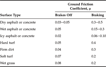
17.2.5 Ground Roll Friction Coefficients
The airplane has to overcome aerodynamic drag and ground friction during the ground roll. The ground friction depends on the weight on wheels and the properties of the ground, which are assessed using the ground roll friction coefficients tabulated below.
17.2.6 Determination of the Lift-off Speed
In this document and unless otherwise specified, the lift-off speed, VLOF, is assumed to be 1.1 times the stalling speed in that particular configuration (e.g. with flaps deployed, landing gear extended, etc.), VS1. Also, VR will be assumed to be about 1.1 times VS1.
If we assume the lift-off speed to be 10% higher than the stalling speed in the T-O configuration, VLOF can be calculated directly using the maximum lift coefficient for the T-O configuration, S for the reference area, and ρ for density as follows:
![]() (17-16)
(17-16)
Most small airplanes lift off as soon as the pilot rotates the airplane at that speed, while larger ones take some 3–5 seconds to lift off after rotation initiates, due to their higher inertia. For the rapid take-off estimation method of Section 17.3.2, Method 2: Rapid T-O distance estimation for a piston-powered airplane, it will be assumed that VR and VLOF are the same value.
Note that determining VLOF and other airspeeds for use in more detailed analysis must comply with regulations. Excerpts that deal with T-O analysis per 14 CFR Part 23 and 25 are provided below.
17.2.7 Determination of Time to Lift-off
The time from brake-release to lift-off can be approximated using the simple expression below, which assumes an average acceleration, a, is known:
![]() (17-17)
(17-17)
If the aircraft is “small,” add 1 second to account for the rotation. If “large,” add 3 seconds.
17.3 Solving the Equation of Motion of the T-O
Now that the equation of motion (EOM) describing the T-O run has been derived, several solution methods will be presented. A solution to the EOM yields information such as the acceleration – average or instantaneous, depending on the solution method – ground run distance, and duration of the ground run. In this section, three methods to estimate the ground run will be introduced to solve the EOM. The first method is a simple solution and is applicable to all aircraft as long as the thrust can be quantified. The second method is intended for piston-powered propeller aircraft only. The third method uses numerical integration to solve the EOM and is, by far, the most powerful of the three.
17.3.1 Method 1: General Solution of the Equation of Motion
This method is applicable to both propeller-powered airplanes as well as jets; the only difference lies in how the thrust is calculated. The method uses Equation (17-4) or (17-5) to calculate the acceleration of the aircraft. With the acceleration in hand, Equation (17-9) is used to estimate the ground run distance. As can be seen, Equations (17-4) and (17-5) both require the estimation of thrust, T, drag, D, and lift, L. The only problem is that all are functions of the airspeed. This therefore begs the question: what airspeed should be used to evaluate them? To answer the question, consider Figure 17-11, which shows how the airspeed of the airplane typically changes during the ground run.
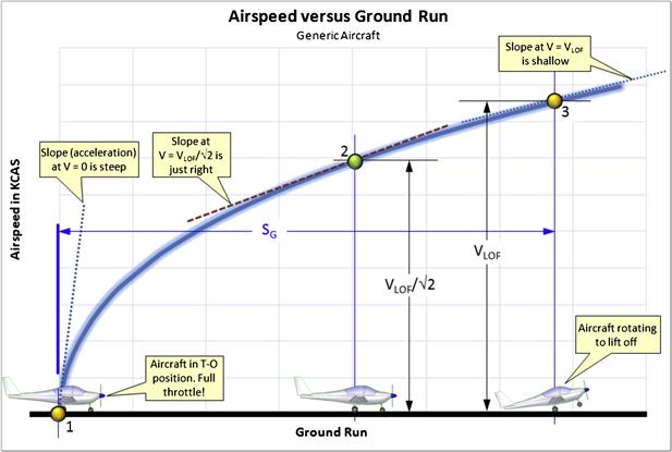
Initially, the acceleration is relatively large, but it gradually diminishes as the airspeed increases. With this in mind, first consider the point labeled ‘1’, but this represents the aircraft in the T-O position, when both V = 0 and SG = 0. It is assumed the engines are allowed to develop full thrust before the airplane begins to accelerate. This way, it achieves maximum acceleration upon brake release (maximum thrust and minimum drag). If the rate of change of speed with distance is denoted with the derivative dV/dS, it is evident that, at this point, it has the steepest slope during the entire ground run. Now consider point ‘3’. This marks the lift-off point and the extent of the ground run. When compared to the start of the ground run, the value of dV/dS has reduced considerably and has reached its lowest value over the entire ground run. It should be clear that if the acceleration at point ‘1’ is used with Equation (17-9), then the estimated ground run will be much less than the actual one, as it is based on a high value of dV/dS. By the same token, if the acceleration at point ‘3’ is used, the ground run estimate will be much larger than experienced, as it is based on a low value of dV/dS. This implies that somewhere between these two extremes exists an airspeed for which the value of dV/dS will give a ground run distance that is in good agreement with experiment. This airspeed is ![]() , where VLOF is the lift-off speed.
, where VLOF is the lift-off speed.
Step 1: Lift-off Speed
Calculate a lift-off speed (VLOF) per Equation (17-16).
Step 3: Lift at the Reduced Lift-off Speed
Calculate lift (L) per Equation (17-10) at![]() .
.
Step 4: Drag at the Reduced Lift-off Speed
Calculate drag (D) per Equation (17-11) at ![]() .
.
Step 5: Thrust at the Reduced Lift-off Speed
Calculate thrust (T) at ![]() , depending on engine type as shown below.
, depending on engine type as shown below.
Thrust for piston-powered aircraft:
![]() (17-18)
(17-18)
Thrust for jet-powered aircraft:
![]() (17-19)
(17-19)
where
PBHP = piston engine horsepower
T() = jet engine thrust function1 using VLOF as an argument
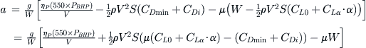
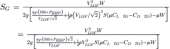
Step 6: Ground Run
Calculate the ground run, using Equation (17-4) or (17-5) with Equation (17-9) of Section 17.2.3, Review of Kinematics, as shown below. Select an appropriate ground friction coefficient, μ, from Table 17-3.
![]() (17-20)
(17-20)
EXAMPLE 17-3
During the T-O phase, the Continental IO-550 engine powering the SR22 generates 310 BHP with an assumed propeller efficiency of 0.65. What is the thrust generated at V = 100 ft/s? What about 120 ft/s (assuming the same propeller efficiency)? If this airplane weighs 3400 lbf, what is the acceleration for both airspeeds (ignoring drag and ground friction)? Discuss the results.
Solution
![]()
![]()
![]()
![]()
These represent absolutely the greatest acceleration the vehicle could possibly have at that condition (assuming the propeller efficiency is valid). The designer should be aware that even though this kind of analysis is simplistic, it serves superbly as a quick “sanity check” when performing a more sophisticated T-O analysis. In this case, it indicates that if using alternative analysis methods, an answer exceeding 10.48 ft/s2 for an SR22 class aircraft is highly suspicious.
EXAMPLE 17-4
The airplane of the previous example is observed to have an average acceleration of 8.74 ft/s2 once it has acquired airspeed of 120 ft/s. If it is assumed this is an “average” acceleration, what distance will the airplane have covered at that airspeed?
Solution
This problem can easily be solved using elementary kinematics:
![]()
This problem is presented as another kind of “sanity check.” The astute aircraft designer will perform such simple and fast checks to evaluate whether errors may have crept into more sophisticated calculations.
EXAMPLE 17-5
Estimate the ground run for a Learjet 45XR using the following properties:
| W = 21,500 lbf S = 311.6 ft2 CL TO = 0.90 CD TO = 0.040 | CLmax = 1.65 T at VLOF/√2 = 7000 lbf μ = 0.02 |
17.3.2 Method 2: Rapid T-O Distance Estimation for a Piston-powered Airplane [5]
This is Method 1 but specifically adapted to the typical piston-engine configuration.
![]() (17-21)
(17-21)
NOTE: If the propeller efficiency, ηP, is not known, the following values can be used as expected approximations:
Derivation of Equation (17-21)
We begin with Equation (17-4) and rewrite the acceleration as follows:
![]() (i)
(i)
Inserting Equations (17-10), (17-11), and (14-38) yields;
Let’s denote the lift and drag coefficients during the T-O run with CL TO and CD TO:
![]() (ii)
(ii)
Insert this into the expression for distance to lift-off to get:
 (iii)
(iii)
Note that since we evaluate the acceleration at ![]() , we incorporate this as follows:
, we incorporate this as follows:
Simplify further:
![]() (iv)
(iv)
Inserting g = 32.174 ft/s2 and arithmetically evaluating the constants leads to:
![]() (v)
(v)
The advantage of this method is that it combines several steps in Method 1, and thus, lends itself better to parametric studies.
QED
EXAMPLE 17-6
Determine the lift-off speed, T-O distance, and time from brake release to lift-off at S-L for the Cirrus SR22 if it has the following characteristics:
| W = 3400 lbf PBHP = 310 S = 144.9 ft2 CLmax = 1.69 (based on POH for T-O) |
CL TO = 0.590 (assumed value) CD TO = 0.0414 (assumed value) μ = 0.04 (sample value) |
Compare the results to published data from the airplane’s pilot’s operating handbook (POH), which gives a lift-off speed of 73 KCAS, T-O distance of 1020 ft (ISA at S-L) and the calculated time to lift-off of 16.6 seconds from EXAMPLE 17-2.
Solution
Lift-off speed:
![]()
Since the propeller efficiency is unknown, let’s pick ηP = 0.50 and calculate lift-off distance:
Note that this example does not account for the rotation, which would add 1 second to the time to lift-off and 118.9 ft to the total distance. This would bring the true ground run SG + SROT to 990 ft, which compares favorably to the POH value of 1028 ft.
17.3.3 Method 3: Solution Using Numerical Integration Method
Since a closed-form integration of Equation (17-4), which accurately accounts for various speed dependencies, is prohibitively hard, it is generally solved numerically. Solving the equation of motion using numerical integration provides the designer with a very powerful technique. When properly applied, the technique even allows time-dependent events to be accounted for during the integration. For instance, consider some specialized T-O technique being modeled in which the flaps are dropped just before lift-off to minimize drag during the ground run. Or, consider the T-O run of many radial piston-powered airplanes of the past. During the ground run, the large radials of many of these old airplanes were operated under limited power until the airplane had accelerated to a certain airspeed, say 60 KIAS. Such complexities are relatively easy to account for using this method. It is the recommended method for serious analysis work.
In this section, we will demonstrate how to setup this method using a spreadsheet. Additionally, the method is very robust as it handles discontinuities with ease, something numerical differentiation schemes would not tolerate as well.
The first step in the scheme is to convert the kinematic Equations (17-7) and (17-8) into the following discrete form:
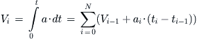 (17-22)
 (17-23)
The variables are depicted in Figure 17-12.
Propeller Thrust at Low Airspeeds
Since the T-O run involves airspeeds ranging from 0 to the lift-off speed, in which the highest acceleration occurs at low speeds, accurate estimation of thrust is imperative. This is problematic for propeller-powered aircraft, where the standard method to extract propeller thrust is that of Equation (14-38), repeated here for convenience:
![]() (14-38)
(14-38)
EXAMPLE 17-7
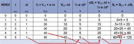
A vehicle accelerates with a constant a = 10 m/s2. Determine its (a) speed, and (b) distance after 5 seconds using numerical integration and compare to the exact solution.
Solution
(a) Numerical integration of the speed: see Figure 17-13.
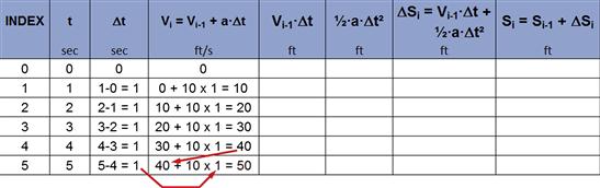
(b) Numerical integration of the distance: see Figure 17-14.
![]()
The inaccuracy is a consequence of a low V and variable and hard-to-predict ηp. This can lead to a thrust estimation that, well, is simply too large. There are two ways to work around this problem. Two methods are presented in Section 14.4.2, Propeller thrust at low airspeeds. One of the two methods is demonstrated in Example 17-8 below.
EXAMPLE 17-8
Determine the lift-off speed, T-O distance, and time from brake release to lift-off at S-L for the Cirrus SR22 by solving the equations of motion using the numerical integration method with the following parameters:
| W = 3400 lbf PBHP = 310 BHP S = 144.9 ft2 Propeller diameter Dp = 76 inches VLOF = 73 KCAS (per POH) |
CLmax = 1.69 (based on POH for T-O) μ = 0.04 (sample value) CL TO = 0.590 CD TO = 0.0414 VH = 186 KTAS (at 2000 ft, per POH) |
Use the method in Section 14.4.2, Propeller thrust at low airspeeds, to approximate the thrust of the constant-speed propeller at low airspeeds. This method approximates the thrust as a function of airspeed using the following cubic spline, reproduced from the above section:
Such a cubic spline will be of the form:
![]() (14-41)
(14-41)
where the constants A, B, C, and D are determined using the following matrix:
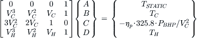 (14-42)
Compare the results to published data from the airplane’s pilot’s operating handbook (POH), which give a lift-off speed of 73 KCAS, T-O distance of 1020 ft (ISA at S-L) and the calculated time to lift-off of 16.6 seconds from EXAMPLE 17-2.
Solution
The solution is implemented as shown in Table 17-4, which was solved using Microsoft Excel. First, focus on the table itself as the reason behind the analysis performed above will become apparent when discussing column 4. Note that the lift-off speed, which is dependent on the CLmax stated above, was calculated in Example 17-6 and found to equal 118.9 ft/s or 70.4 KCAS. This serves as a flag in the calculations below – once the airspeed is greater than 118.9 ft/s, the ground run is assumed completed.
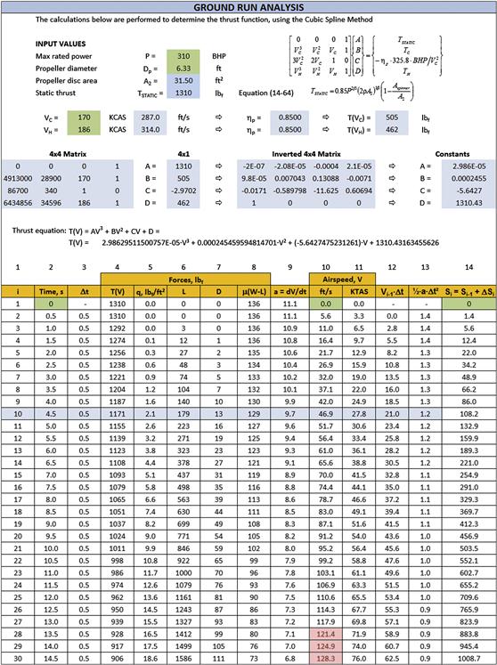
In order to help explain steps required to setup the spreadsheet, the columns have been numbered from 1 through 15. The first column (i) lists the indexes used, here ranging from 1 through 30. Effectively, all rows from 2 through 30 contain the same formulas, but row 1 differs as it is required to contain the initial conditions.
Column 1 is the index ‘i’ shown in Equations (17-22) and (17-23). Note the row with the index ‘10’ has been shaded to draw attention to it as it is used as an example of calculations.
Column 2 is the time. Here, the event starts when t = 0 sec and ends when t = 20 sec. The initial time (when i = 1) is zero by definition. All subsequent times are obtained by simply adding 0.5 sec to the value in the cell above. It is ultimately the user’s decision how many rows to use to represent a time interval in which the event (T-O ground run) takes place.
Column 3 is the time step. Note that each row represents a specific time step, Δt, in the analysis. Here all the time steps are equal. Thus the 10th time step (when i = 10) takes place when t = 4.5 sec. It is recommended that the method is implemented using 0.25 sec or 0.5 sec time steps. The time step is simply calculated by subtracting the previous time from the current time. Thus, the time step in row 10 is obtained by Δt = 4.5 − 4.0 = 0.5. The same result is obtained for the other rows, except the first one, as it does not have a preceding time. Note that even though each time step in the table is 0.5 second, it does not have to be so; time steps can be of variable size. This allows higher definition around a specific event of interest. For instance consider modeling flaps being deployed sometime during the ground run over a period of time. It is appropriate to relax time steps before and after events that take place during the T-O run and use smaller time steps as deemed appropriate.
Column 4 is the propeller thrust force. It is calculated using the cubic spline method presented in method 3 of Section 14.4.2, Propeller thrust at low airspeeds. The method creates a cubic polynomial that is a function of time. Its general form is T(V) = AV3 + BV2 + CV + D, where A, B, C, and D are determined based on the static thrust, TSTATIC, and the airspeeds VC and VH, and the thrust at those airspeed, denoted by TC and TH. The airspeed, denoted by V, is obtained from column 11. Note that in order to prevent circular error, the value of V is taken from the previous row. Thus, the value of V used in row 10 is that calculated in row 9.
Column 5 is the dynamic pressure, here calculated using density at S-L and the airspeed from column 11. The value of V in Row 10 is taken from Row 9 in order to prevent circular error from occurring in Microsoft Excel. The difference is dynamic pressure is considered acceptable, although it highlights why the time steps should be as small as practical. The dynamic pressure in Row 10 is 2.1 lbf/ft2.
Column 6 is the lift force, here calculated using density at S-L, the airspeed from column 11, a wing area of 144.9 ft2, and the CL TO given in the problem statement. Calculated from L = q·S·CL TO. The lift in row 10 is 179 lbf.
Column 7 is the drag force, using the same parameters as for column 6, with the exception of the drag coefficient given by CD TO. Calculated from D = q·S·CD TO. The drag force in row 10 is 13 lbf.
Column 8 is the ground friction force, using the values from column 6, the weight (3400 lbf), and the ground friction constant μ, given in the problem statement. Calculated from μ·(W-L). The ground friction in row 10 is 129 lbf.
Column 9 is the acceleration. Calculated by summing the forces and dividing by the mass. The mass is simply the weight divided by the acceleration due to gravity, g = 32.174 fts2. Calculated from:
![]()
Thus, the acceleration in row 10 is obtained as follows:
![]()
Columns 10 and 11 is the airspeed. The value in column 10 is calculated using the simple kinematic expression of Equation (17-22), i.e.: Vi = Vi−1 + ai·Δti. Using row 10 as an example, V9 = 42.0 ft/s, a10 = 9.74 ft/s2, and Δt10 = 0.5 sec. Therefore, V10 = V9 + a10·Δt10 = 43.1 + 9.74·0.5 = 46.9 ft/s. The value in column 11 amounts to Vi/1.688, converting ft/s to knots.
Columns 12 through 15 form the distance calculations shown in Equation (17-23). Column 12 is calculated from the expression Vi−1 ·Δti. Thus, row 10 is calculated from V9 ·Δt10 = 42.0·0.5 = 21.0 ft. Column 13 is calculated from the expression ½·ai−1·(Δti)2, which for row 10 translates to ½·a9·(Δt10)2 = ½·9.7·(0.5)2 = 1.2 ft. Column 14 is calculated using the expression Si = Si-1 + Vi-1 ·Δti + ½·ai−1·Δti2, which for row 10 becomes: S10 = S9 + V9 ·Δt10 + ½·a9·Δt102 = 86.0 + 21.0 + 1.2 = 108.2 ft. This represents the cumulative distance up to that point in time.
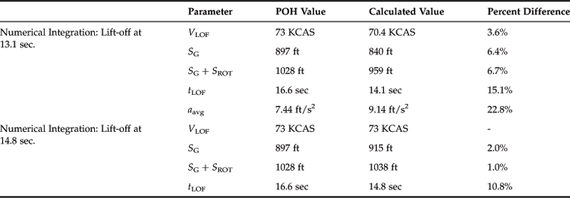
With these explanations behind us, it is now possible to explore some of the results. Table 17-4 shows that the airplane accelerates to lift-off speed between rows 27 and 28 (between 13.0 and 13.5 seconds). Interpolating between these two values yields t = 13.1 seconds and SG = 840 ft. Adding the rotation segment, the distance increases by SROT = |VLOF| = 119 ft, yields a total ground run of 959 ft, and time to lift-off is 14.1 seconds. The distance is 61 ft shorter than the POH figure. On the other hand, if the airplane is allowed to accelerate to 73 knots, as the POH states, the time to lift-off speed is t = (13.8 + 1) sec and SG = 915 ft, leading to a total distance of 1038 ft (note that 73 knots is about 123 ft). Other numbers are compared in Table 17-5 below.
Considering other results, Figure 17-15 shows the thrust and propeller efficiency models used for this analysis. The shaded region in the graph represents the focus of the above work and shows that the cubic spline method allows the thrust to be determined to a zero airspeed.
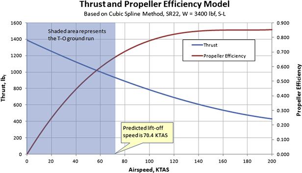
FIGURE 17-15 The thrust and propeller efficiency model for the SR22 used in the T-O ground run analysis.
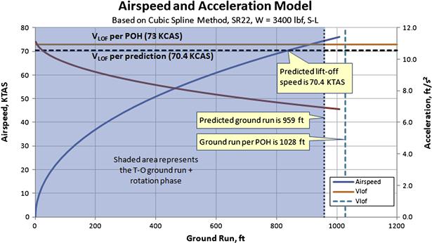
The ground run numbers in the POH for the SR22 includes the rotation phase, which here is assumed to be 1 second. Therefore, a 1-second rotation segment is added to the POH value for the ground run analysis. Consequently, the comparable POH ground run should be 1020 – 123 = 897 ft. It is also possible to adjust the time for lift-off by subtracting the 1 second from the 16.6 sec in EXAMPLE 17-2. From the graph we can see that VLOF calculated (70.4 KCAS) using 1.1VS is a tad slower than the value found in the POH (73 KCAS). Therefore, a comparison assuming that airspeed is included as well. The conclusion is that based on the average acceleration, there are some parameters of the prediction that might be improved with an adjustment. For instance, it is possible that the predicted static thrust is too high, although it included the empirical reduction factor discussed in Section 14.5.3, Maximum static thrust. Also, it is possible that drag for the T-O configuration is underestimated, and so on. Regardless, if the lift-off speeds (73 KCAS actual versus the predicted 70.4 KCAS) are comparable, the method and experiment are likely to agree well (see Figure 17-16).
17.3.4 Determination of Distance During Rotation
Figure 17-17 shows an aircraft taking off and clearing an obstruction of predetermined height shortly after lift-off. Refer to this figure for the remaining segments of the T-O run, starting with the rotation. Rotation is a very transient event during the T-O. Small airplanes lift off almost as soon as the pilot initiates the rotation (by deflecting the elevator to raise the nose). For large, heavy aircraft the rotation may last anywhere from 2 to 5 seconds. Accounting for the change in drag and lift during the rotation can be implemented using the numerical integration scheme; however, it is far simpler to account for distance traveled during rotation by assuming the distance a small aircraft travels in 1 second, and a large aircraft in 3 seconds. Mathematically:

It is recognized that the boundary between “small” and “large” aircraft is somewhat subjective, but it is somewhere between a Beech 99 King Air and a British Aerospace BAe 146, with a Fokker F-27 or F-50 in that gray area.
17.3.5 Determination of Distance for Transition
Referring again to Figure 17-17, the transition segment begins with the lift-off and ends with the aircraft achieving a climb angle to be maintained until the obstacle height is achieved. As stated earlier, we want to determine the total distance from the lift-off point to the location where the airplane clears the obstacle, call it Sobst. There are typically two issues that one must contend with when determining this distance: is the obstacle cleared before or after the transition segment is completed? A methodology to evaluate the distance denoted by Sobst will now be presented. Refer to Figure 17-18 for a more detailed look at this scenario. The following parameters are essential to the analysis of this phase of the T-O maneuver:

FIGURE 17-18 Evaluation of the T-O over an obstacle. The left image shows the aircraft crossing the obstacle after transitioning from the curved into the straight climb. In this case the climb segment must be added to the total. The right image shows the aircraft crossing before it transitions. Only the distance to where it reaches hobst is needed and no climb calculations are necessary.
Climb angle:
![]() (18-20)
(18-20)
Transition distance:
![]() (17-26)
(17-26)
Transition height:
![]() (17-27)
(17-27)
Derivation of Equations (17-26) and (17-27)
Transition generally implies acceleration from 1.1VS1 to a climb speed of 1.2VS1. Note that the climb speed may not necessarily be the best rate of or best angle of climb for the airplane. The average speed for the two limits is of course 1.15VS1 and this is used in addition to an assumed lift coefficient of about 0.9CLmax to determine distance traveled as follows:
Step 1: Average vertical acceleration in terms of load factor.
![]() (17-28)
(17-28)
Step 2: Use the load factor to determine the radius of the curved segment, by using the expression for the centripetal acceleration required. Load factor in terms of centripetal force:
![]()
Step 3: Determine the angle through which the rotation takes place using Equation (18-20) by solving for θ.
Step 4 – Transition occurs BELOW obstacle height: refer to Figure 17-18, the left part of which shows a schematic of the initial climb in which the aircraft clears the obstacle after transitioning from the curved into the straight climb. In this case, the straight climb segment must be added to the total T-O distance. The trick is to determine STR and SC. Here, the combination of the two is denoted by Sobst. By inspection it can be seen that the horizontal distance (STR) must equal R·sin θclimb and the altitude gained (hTR) during the transition amounts to R·(1 − cos θclimb). These are expressed in Equations (17-26) and (17-27).
Step 4 – Transition occurs ABOVE obstacle height: the right part of Figure 17-18 shows the aircraft passing the obstacle before completing the transition. Consequently, we only need to determine the distance to where it cleared the obstacle and no climb calculations are needed. This distance, again, is denoted by Sobst. It can be seen that the horizontal distance (STR) is given by the Pythagorean rule:
![]() (17-31)
(17-31)
Therefore, the distance required to clear the obstacle can be approximated by considering the ratio between the height and
![]() (17-32)
(17-32)
QED
17.3.6 Determination of Distance for Climb Over an Obstacle
As stated above, if the value of hTR is less than the obstacle height, the airplane covers additional distance while climbing. The required obstacle clearing height is 50 ft for military and GA aircraft, and 35 ft for commercial aircraft. This distance can be observed from Figure 17-18 as follows:
![]() (17-33)
(17-33)
EXAMPLE 17-9
Determine the transition distance and, if found necessary, the climb distance for the Cirrus SR22. Use data from Example 17-8 as needed. Assume the simplified drag model and the following characteristics:
| W = 3400 lbf S = 144.9 ft2 CLmax = 1.69 (based on POH for T-O) |
CDmin = 0.0350 (T-O configuration, assumed) k = 0.04207 |
Compare the results to published data from the airplane’s Pilot’s Operating Handbook (POH), which gives a lift-off speed of 73 KCAS, T-O distance of 1020 ft (ISA at S-L) and the calculated time to lift-off of 16.6 seconds from Example 17-2.
Solution
![]()
![]()
![]()
![]()
![]()
![]()
![]()
![]()
![]()
![]()
Since the hTR is less than the obstacle height of 50 ft, the climb segment must be included as well.
Therefore, the total T-O distance over 50 ft is 959 + 467 + 33 = 1459 ft, if the estimated VLOF of 70.4 KCAS is used, and 1038 + 467 + 33 = 1538 ft, if the POH VLOF of 73 KCAS is used. The numbers compare to 1594 ft in the POH.
17.3.7 Treatment of T-O Run for a Taildragger
Fundamentally, only the ground run analysis for a taildragger differs from that of a conventional tricycle aircraft. This is because early in the ground run the taildragger can lift its tailwheel off the ground, effectively rendering it a different aircraft configuration. How quickly this happens depends on the aircraft itself. Some taildraggers generate enough thrust to lift the tail as soon as the engine power is increased. Others must accelerate to some airspeed before enough lift is generated by the HT to raise the tailwheel.
For this reason, the taildragger must really be considered as two separate configurations: one has the tailwheel on the ground and the other off the ground. Each configuration is subject to different lift and drag coefficients. It is easiest to treat the T-O run using the numerical method of Section 17.3.3, Method 3: Solution using numerical integration method. This will even permit a transition to be incorporated, i.e. the lift-and-drag coefficients are functions of the AOA of the vehicle, which changes from the tail-on-ground angle to tail-off-ground angle over a period of 1 or 2 seconds. The airspeed at which this takes place can be calculated using the method from Section 13.3.5, Taildragger landing gear reaction loads.
17.3.8 Take-off Sensitivity Studies
Once the proper formulation for the T-O run has been prepared, it is helpful to study the impact of variation in atmospheric conditions, weight, runway slope, and other deviations on the operation of the airplane. Three examples of sensitivity studies have been prepared for the SR22 and are shown in Figure 17-19, Figure 17-20, and Figure 17-21. The first one is the sensitivity of the T-O distance to changes in temperature and altitude. Among other things, it shows that a T-O from an airfield at a 10,000 ft elevation on a standard day results in a doubling of the T-O distance over 50 ft. On a day that is 30 °C hotter the distance increases by a factor of 2.7.
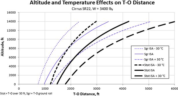
FIGURE 17-19 Sensitivity study showing the effect of altitude and temperature on the T-O distance of the SR22. The study was performed using the analysis method presented in this section.
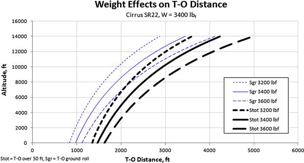
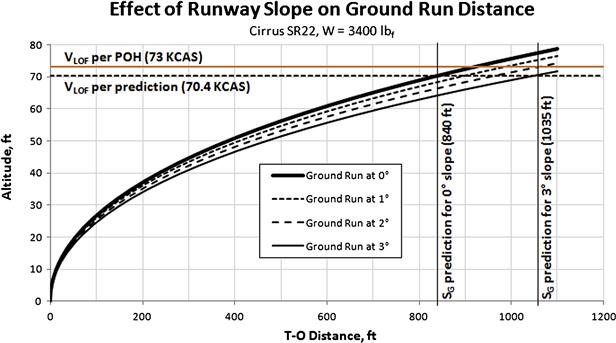
FIGURE 17-21 Sensitivity study showing the effect of runway slope change on the T-O distance of the SR22.
The sensitivity being studied in Figure 17-20 shows how weight and altitude affect the T-O distance. A study of this nature is helpful when evaluating the impact of a target gross weight not being met. Generally, increasing the gross weight by 200 lbf will increase the ground run distance by 150 to 675 ft and T-O over 50 ft by 155 to 750 ft, depending on altitude.
The impact of a steep runway slope is presented in Figure 17-21 and is based on Equation (17-5). The figure shows that an uphill runway slope of some 3° will increase the ground run distance by almost 200 ft, from 840 ft to 1035 ft. While this information is helpful for some preliminary design studies, it is vital for the pilot once the aircraft is operational. Most runways feature some degree of uphill or downhill slope; understanding the detrimental effect of uphill slopes, in particular, helps the pilot in the decision-making process.
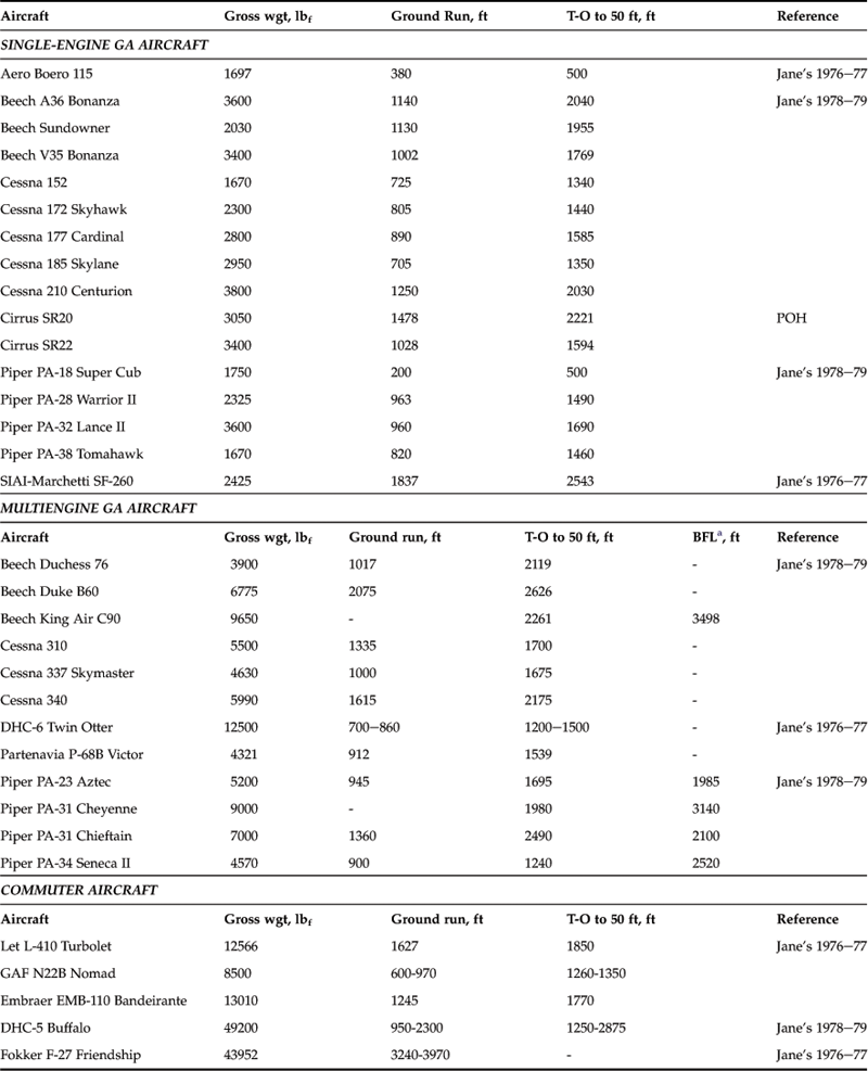
17.4 Database – T-O Performance of Selected Aircraft
Table 17-6 shows the ground run and T-O distance to reach 50 ft altitude above ground level. This data is very helpful when evaluating the accuracy of own calculations.
Exercises
(1) The six-seat Beech B58 Baron has two 260 BHP Continental IO-470 engines that swing 78-inch diameter propellers. Its gross weight is 5100 lbf, and it has a 199.2 ft2 wing area and a 37.83 ft wing span. Estimate its balanced field length at S-L on a standard day, assuming the maximum lift coefficient in the T-O configuration to is 1.60, minimum drag coefficient is 0.035, lift-induced drag constant is 0.05906, and V2 = 1.2VS for an obstacle height of 50 ft. Assume the simplified drag model. Assume the maximum thrust with one engine inoperable (OEI) to equal one half of the average T-O thrust. Compare your number to the published value of about 2300 ft.
(2) Estimate the average acceleration and time from break release to lift-off for the following aircraft types, based on the ground run and lift-off speed specified in their pilot’s operating handbooks (assume S-L conditions).
(a) Beechcraft B58 Baron, SG = 2000 ft, VLOF = 84 KCAS.
(b) SOCATA TBM-850, SG = 1017 ft, VLOF = 77 KCAS.
(c) Cessna C-208 Grand Caravan, SG = 1405 ft, VLOF = 86 KCAS.
(d) Piper PA-46 Malibu Mirage, SG = 1100 ft, VLOF = 69 KCAS.
(3) Estimate the ground run for the three-engine Dassault Falcon 7X business jet, using the following properties:
| W = 70,000 lbf S = 761 ft2 CL TO = 0.85 CD TO = 0.045 | CLmax = 1.5 T at VLOF/√2 = 3 × 6000 lbf μ = 0.03 |
(4) Determine the lift-off speed (VLOF), V2, and total T-O distance to an obstacle height of 50 ft (includes ground roll, rotation, transition, and climb distances) for the turboprop-powered SOCATA TBM-850, assuming the following characteristics:
| W = 7394 lbf P = 850 SHP (PT6A) S = 193.7 ft2 CLmax = 1.90 (based on POH for T-O) | CL TO = 0.750 (assumed value) CD TO = 0.045 (assumed value) μ = 0.03 (sample value) ηp = 0.65 |
Compare the results to published data from the airplane’s pilot’s operating handbook (POH), which gives a VLOF = 90 KCAS, V2 = 99 KCAS, ground roll distance of 2035 ft (ISA at S-L) and total T-O distance (to 50 ft) of 2840 ft.

References
1. Perkins CD, Hage RE. Airplane Performance, Stability, and Control. John Wiley & Sons 1949.
2. Torenbeek E. Synthesis of Subsonic Aircraft Design. 3rd ed. Delft University Press 1986.
3. Nicolai L. Fundamentals of Aircraft Design. 2nd ed. 1984.
4. Roskam J, Lan Chuan-Tau Edward. Airplane Aerodynamics and Performance. DARcorporation 1997.
5. Hale FJ. Aircraft Performance, Selection, and Design. John Wiley & Sons 1984; pp. 137–138.
6. Anderson Jr JD. Aircraft Performance & Design. 1st ed. McGraw-Hill 1998.
1For jet engines, this is typically obtained using the engine manufacturer’s engine deck.