
Performance – Range Analysis
Abstract
The chapter presents the fundamental theory of range analysis, as well as information required to complete such analysis. It is shown that classic range analysis methods can be used for at least three disparate cruise profiles for aircraft powered by fossil fuels, and one for aircraft that use electric power. These profiles are referred to as a constant airspeed/altitude, constant attitude/altitude, constant airspeed/attitude, and constant weight profiles, respectively. Range sensitivity is also introduced. Then, the concept of specific range is discussed. This is followed by the presentation of some classic endurance analysis methods in a manner similar to that for range analysis. Then methods that are useful to the analysis of aircraft mission profiles are introduced, but these are needed to determine realistic fuel requirements for the new aircraft. The chapter also introduces two important and common mission profiles to which many GA aircraft are designed; the standard IFR cruise mission and NBAA cruise mission. Finally, an introduction to payload-range analysis is provided.
Keywords
Range; endurance; Breguet range; Breguet endurance; cruise segment; initial weight; final weight; fuel weight; specific fuel consumption; thrust specific fuel consumption; SFC; constant airspeed/constant altitude; constant altitude/constant attitude; constant airspeed/constant attitude; sensitivity; specific range; NBAA range; IFR range; range efficiency; CAFÉ; mission profile; mission range; weight ratio; payload-range
Outline
20.1.1 The Content of this Chapter
20.1.2 Basic Cruise Segment for Range Analysis
20.1.3 Basic Cruise Segment in Terms of Range Versus Weight
20.1.4 The “Breguet” Range Equation
20.1.5 Basic Cruise Segment for Endurance Analysis
20.1.6 The “Breguet” Endurance Equation
Thrust Specific Fuel Consumption for a Jet
Thrust Specific Fuel Consumption for a Piston Engine
20.2.2 Range Profile 1: Constant Airspeed/Constant Altitude Cruise
Derivation of Equation (20-10)
20.2.3 Range Profile 2: Constant Altitude/Constant Attitude Cruise
Derivation of Equation (20-11)
20.2.4 Range Profile 3: Constant Airspeed/Constant Attitude Cruise
Derivation of Equation (20-12)
20.2.5 Range Profile 4: Cruise Range in the Absence of Weight Change
20.2.6 Determining Fuel Required for a Mission
Range Profile 1: Constant Airspeed/Altitude Cruise
Derivation of Equation (20-14)
Range Profile 3: Constant Airspeed/Attitude Cruise
Derivation of Equation (20-15)
20.2.7 Range Sensitivity Studies
20.3.2 CAFE Foundation Challenge
20.4 Fundamental Relations for Endurance Analysis
20.4.1 Endurance Profile 1: Constant Airspeed/Constant Altitude Cruise
Derivation of Equation (20-19)
20.4.2 Endurance Profile 2: Constant Attitude/Altitude Cruise
Derivation of Equation (20-20)
Derivation of Equation (20-21)
20.4.3 Endurance Profile 3: Constant Airspeed/Attitude Cruise
Derivation of Equation (20-22)
20.5 Analysis of Mission Profile
20.5.1 Basics of Mission Profile Analysis
Weight ratios for selected segments
20.5.2 Methodology for Mission Analysis
20.5.3 Special Range Mission 1: IFR Cruise Mission
20.5.4 Special Range Mission 2: NBAA Cruise Mission
20.1 Introduction
The majority of aircraft are designed to carry people or freight from a place of origin to some destination. Such airplanes emphasize range or endurance above other characteristics. While aircraft are certainly designed to satisfy other requirements, such as that of speed or maneuverability, range and endurance are almost always included as some of the most important ones. Even the fastest and most maneuverable aircraft would not amount to much if it didn’t also offer acceptable range or endurance. In this section we will present methods to estimate range and endurance for aircraft.
Range is the distance an airplane can fly in a given time. This distance is of great importance in aircraft design and is often the parameter used to determine whether a particular design is viable. The range can be broken into a basic segment, called a cruise segment, during which some specific boundary conditions are established. Such boundary conditions allow the amount of energy required (i.e. fuel) to be evaluated. This evaluation impacts the weight requirements for that aircraft, which, in turn, impacts its size, and so on. Figure 20-1 shows how range analysis fits among the other branches of Performance theory.
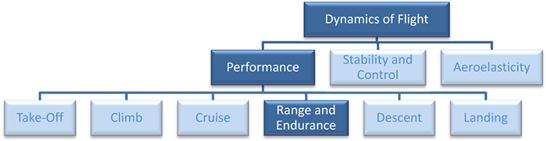
FIGURE 20-1 An organizational map placing performance theory among the disciplines of dynamics of flight, and highlighting the focus of this section: range and endurance.
In general, the methods presented in here are the “industry standard” and mirror those presented by a variety of authors, e.g. Perkins and Hage [1], Torenbeek [2], Nicolai [3], Roskam [4], Hale [5], Anderson [6] and many, many others.
20.1.1 The Content of this Chapter
• Section 20.1 presents fundamental theory of range analysis, as well as information required to complete such analysis.
• Section 20.2 presents classic range analysis methods using three different cruise profiles for aircraft powered by fossil fuels, and one aimed at aircraft that use electric power. These profiles are referred to as a constant airspeed/altitude, constant attitude/altitude, constant airspeed/attitude, and constant weight profiles, respectively. The end of the section presents methods to evaluate range sensitivity.
• Section 20.3 presents the concept of specific range.
• Section 20.4 presents classic endurance analysis methods in a manner similar to that for range analysis.
• Section 20.5 presents methods to analyze the mission profile of the aircraft, but these are needed to determine realistic fuel requirements for the new aircraft. The section also introduces two important and common mission profiles to which many GA aircraft are designed; the standard IFR cruise mission and NBAA cruise mission. The section also presents the important payload-range analysis.
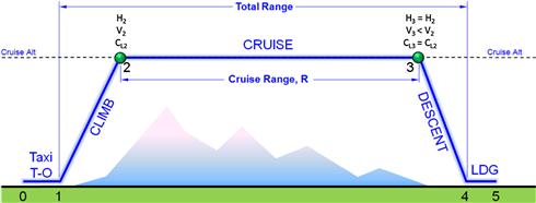
20.1.2 Basic Cruise Segment for Range Analysis
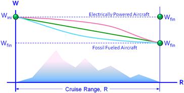
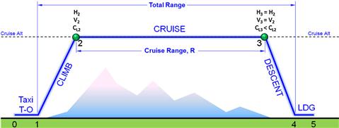
The basic cruise segment is shown in Figure 20-2. The aircraft begins the cruise at some initial weight, Wini, and after covering some distance, R, will now possess some final weight, Wfin. This weight is less than the initial weight if the aircraft is powered by engines that burn fossil fuel, but unchanged if the source of energy is electric power. Both energy sources will be considered in this chapter. Note that the three curves in the figure indicate the aircraft may initially burn more (blue curve) or less fuel (lavender curve) than later in the segment. However, for simplicity, it is often assumed the fuel burn is pretty much linear for the segment and this approximation is in fact accurate (straight line). It is customary to break segments of hugely varying fuel consumption into smaller segments for which the linear assumption holds.
20.1.3 Basic Cruise Segment in Terms of Range Versus Weight
For mathematical convenience it is useful to transpose the axes in Figure 20-2 to what is shown in Figure 20-3. In this figure the weight becomes the horizontal axis and the range the vertical one. It is evident that the range changes from 0 at Wini to the final range, Rfin, at Wfin.

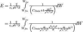
From this we can define the change in range as follows:
![]() (20-1)
(20-1)
where
During cruise it is reasonable to assume that T = D and D = W/(L/D). For this reason we can rewrite the change in range as follows:
![]() (20-2)
(20-2)
Note that expressions (20-1) and (20-2) are only valid for aircraft that burn fuel. An expression for electrically powered aircraft does not depend on the change in weight.
20.1.4 The “Breguet” Range Equation
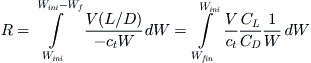
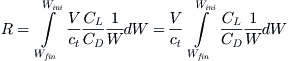
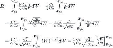
Equation (20-2) is solved for the range by integration, in which the limits are the initial and final weight during that segment. This equation was developed by the French aircraft designer Louis Charles Breguet (1880–1955), who was one of the early pioneers of aviation. Therefore, it is referred to as the “Breguet” range equation:
 (20-3)
In order to solve Equation (20-3) we must incorporate the dependency of V, L/D, and ct on W, but these are established in accordance with what “kind” of a cruise we intend to fly. The Breguet equation lends itself well to numerical integration. However, it is common to give closed-form solutions to problems using some simplifying assumptions. All such solutions assume that the specific fuel consumption is constant and an “average” value for the entire range can be determined. Several well known closed-form solutions of the Breguet equation are provided in Section 20.2, Range analysis. Section 20.2.5, Range profile 4: cruise range in the absence of weight change, provides a method to handle range in the absence of weight change (for electrically powered aircraft).
20.1.5 Basic Cruise Segment for Endurance Analysis
Endurance is the length of time an airplane can stay aloft while consuming a specific amount of fuel. Like range, this length of time is of great importance in aircraft design, particularly for some military aircraft, such as fighters, tankers, and UAVs. As in the case of the range, endurance is considered in terms of a cruise segment, during which some specific boundary conditions are established that are then used to evaluate this parameter. Such a segment is shown in Figure 20-4 and is identical to Figure 20-3, except that the vertical axis features time.

Begin by defining the thrust specific fuel consumption as follows:
![]() (20-4)
(20-4)
The inverse of the term dW/dt is simply the rate of change in time with respect to weight. This allows us to write the change in time aloft as follows:
![]() (20-5)
(20-5)
Expand this expression by introducing the same assumptions as for the range, i.e. noting that T = D = W/(L/D) as done for Equation (20-2), which yields:
![]() (20-6)
(20-6)
In order to solve Equation (20-6) we must incorporate the dependency of V, L/D, and ct on W.
20.1.6 The “Breguet” Endurance Equation
As for the range, Equation (20-6) is solved for the endurance by integration, in which the limits are the initial and final weight during that segment. It is referred to as the “Breguet” endurance equation:
 (20-7)
The solution of Equation (20-7) requires the dependency of V, L/D, and ct on W to be established in the same manner as for the range. As before, closed-form solutions exist for the same cases as for the range and are based on similar assumptions. All of the closed-form solutions given below assume the simplified drag model of Chapter 15.
20.1.7 Notes on SFC and TSFC
Thrust Specific Fuel Consumption for a Jet
In the UK system, the specific fuel consumption (cjet) for a jet is given in terms of lbf/hr/lbf. But since V is in terms of ft/s the units must be made consistent.
![]()
Therefore, the TSFC for a jet is given by (unit is 1/s or lbf/sec/lbf):
![]() (20-8)
(20-8)
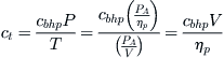
Thrust Specific Fuel Consumption for a Piston Engine
In the UK system, the specific fuel consumption (cbhp) for a piston engine is given in terms of lbf/hr/BHP (in terms of power). So, it must be converted to reflect thrust specific fuel consumption. The resulting expression for the TSFC for a piston engine aircraft is given by (units is 1/s):
![]() (20-9)
(20-9)
Derivation of Equation (20-9)
![]() (i)
(i)
![]() (ii)
(ii)
![]() (iii)
(iii)
The available power, call it PA, is related to the available engine power as follows:
![]() (iv)
(iv)
However, PA can also be written as:
![]() (v)
(v)
Inserting Equations (iv) and (v) into Equation (iii) yields:
 (vi)
(vi)
Consider the units for Equation (vi):

For proper results, the dependency of the SFC on hours and BHP must be eliminated. To do this, divide by 60 × 60 = 3600 sec/hr and 550 ft·lbf/sec. Thus, Equation (vi) becomes:
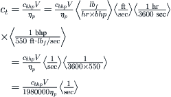
QED
20.2 Range Analysis
Range analysis is an investigation of how far an aircraft can fly, how quickly, and at what cost. The analysis does not only consider what airspeed an airplane must maintain in order to obtain optimum range, but also evaluates what impact it has when other airspeeds are chosen. It also allows various sensitivities to be evaluated, such as the effect of fuel weight.
20.2.1 Mission Profiles
Generally, airplanes follow three different types of operation during cruise, based on selected combinations of the following physical and mathematical interpretations. These are shown in Table 20-1.
TABLE 20-1
Physical and Mathematical Interpretation of Parameters for Mission Analysis
| Physical Interpretation | Mathematical Interpretation |
| Constant airspeed implies… | … V = Constant |
| Constant altitude implies… | … ρ = Constant |
| Constant attitude (i.e. AOA) implies… | … CL/CD = Constant |
Closed-form solutions are provided for the combinations of parameters in Table 20-2.

It is helpful to keep Equation (9-47) in mind when considering these combinations, repeated here for convenience:
![]() (9-47)
(9-47)
20.2.2 Range Profile 1: Constant Airspeed/Constant Altitude Cruise
This type of cruise requires the airspeed and altitude to be maintained between Points 2 and 3 (the cruise segment) in Figure 20-5. Since the weight of the airplane reduces with time as fuel is consumed, this requires the AOA or the attitude of the aircraft to be reduced accordingly. Reducing the AOA reduces the lift coefficient, which, as can be seen from Equation (9-47), is the only way to reduce the lift if V and ρ are constant. Note that Equation (20-10) below only yields the distance covered between Points 2 and 3.
Cruise Type 1
![]() (20-10)
(20-10)
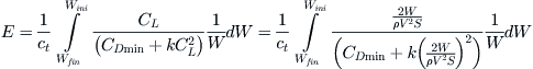
Derivation of Equation (20-10)
In all three cases, the thrust specific fuel consumption, ct, is constant. Additionally for this case, the airspeed, V, is also constant. However, since CL/CD is dependent on the change in weight this must remain inside the integral. Therefore, we write Equation (20-3) as follows:
Insert the expression for drag (here using the simplified drag model of Equation (15-5) to get:
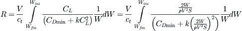

Expanding further leads to:

QED
EXAMPLE 20-1
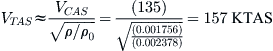
A light airplane starts its cruise segment at 150 KTAS at 10,000 ft when it weighs 3200 lbs. After cruising for a period of time at that altitude it is noticed it now weighs 2800 lbs.
Using a wing area of S = 145 ft² compute the initial and final lift coefficients if the pilot maintains constant airspeed.
20.2.3 Range Profile 2: Constant Altitude/Constant Attitude Cruise
This type of cruise requires the altitude and attitude (AOA) to be maintained between Points 2 and 3 (the cruise segment) in Figure 20-6. Since the weight of the airplane reduces with time as fuel is consumed, this requires the airspeed of the aircraft to be reduced and this, as can be seen from Equation (9-47), is the only way to reduce the lift (since CL and ρ will not change). Note that Equation (20-11) below is the distance covered between Points 2 and 3.
Cruise Type 2
Airspeed – must be reduced during cruise (V = Variable)
![]() (20-11)
(20-11)
Derivation of Equation (20-11)
For this case, the airspeed, V, is a variable and CL/CD is a constant and, thus, can come outside the integral.
Therefore:
![]()
QED
EXAMPLE 20-2
The light airplane of EXAMPLE 20-1 again starts its cruise segment at 150 KTAS at 10,000 ft when it weighs 3200 lbs. After cruising for a period of time at that altitude it is noticed it now weighs 2800 lbs.
Using a wing area of S = 145 ft² compute the final airspeed if the pilot maintains a constant lift coefficient.
20.2.4 Range Profile 3: Constant Airspeed/Constant Attitude Cruise
The third cruise profile is the constant airspeed/constant attitude cruise. In this cruise mode, the airplane must climb as the fuel is consumed to ensure less lift is generated (per Equation (9-47)) at the constant airspeed between Points 2 and 3 (the cruise segment) in Figure 20-7. Note that Equation (20-12) below is the distance covered between Points 2 and 3.
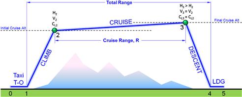
Cruise Type 3
Airspeed – constant during cruise (V = Constant)
Altitude – increases during cruise (ρ = Variable)
AOA – constant during cruise (L/D = Constant)
![]() (20-12)
(20-12)
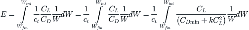
Derivation of Equation (20-12)
For this case, the airspeed, V, and CL/CD are constant and, thus, can come outside of the integral.

QED
EXAMPLE 20-3
The light airplane of Example 20-1 again starts its cruise segment at 150 KTAS at 10,000 ft when it weighs 3200 lbs and cruises for a period of time until it weighs 2800 lbs.
Using a wing area of S = 145 ft² compute the final density altitude if the pilot maintains a constant airspeed and AOA. Compute dynamic pressure at the beginning and end of the cruise.
20.2.5 Range Profile 4: Cruise Range in the Absence of Weight Change
At the time of writing, electric airplanes capable of carrying people are steadily gaining popularity. The advent of batteries with high enough energy density to be practical for use in such aircraft is likely to change the face of aviation in the future. Airplanes powered with solar energy are being developed and a number of such airplanes have already flown. Electric airplanes differ from the aircraft of previous sections in that their weight does not change with range or, in the case of fuel cells, changes very slightly. For this reason the Breguet formulation is not applicable. This section will focus on how to compute the range of airplanes powered by electric motors driven by batteries. It is assumed the airplane flies at a constant altitude. For this particular section it is assumed the profile of Figure 20-5 applies.
Let mb be the mass (or weight) of the battery system and let EBATT be the energy density of the battery. Then the total energy stored in the battery system will be E = mb × EBATT. Suppose the power of the motor is PELECTRIC, then the time to run the motor is:
![]() (20-13)
(20-13)
In order to determine maximum range, the designer should tabulate the power required for a range of airspeeds as set up in Table 20-3 below and then extract the best range. Note that PREQ is the power the electric motor must generate and is thus a direct indication of the power setting required. Also, although not directly shown in the table, it is assumed the proper conversion factors are employed to ensure the units displayed.
EXAMPLE 20-4
An electric airplane is being designed to feature 200 kg of lithium polymer (LiPo) batteries. Its electric motor is rated at 60 kW at full power (or 60,000 W). If the energy density is 130 Wh/kg and the airplane’s minimum power required is 10,000 ft·lbf/s at the intended cruise altitude, determine the percentage power required and endurance. If the minimum power airspeed is 83 KTAS, determine the range. Note that disparate units are being used for demonstration purposes only.
EXAMPLE 20-5
Consider a Cirrus SR22 as it begins its cruise segment at 135 KCAS at 10,000 ft, weighing 3200 lbf, and cruises for a period of time at that altitude until it weighs 2800 lbf. The following additional data is given:
| Wing area | S = 145 ft² |
| Aspect ratio | AR = 10 |
| Minimum drag coefficient | CDmin = 0.025 |
| Average fuel burn | 15 gallons/hr |
| Average BHP | 150 BHP |
| Propeller efficiency | ηp = 0.85 |
Compute the range of this airplane using each of the three cruise profiles.

EXAMPLE 20-6
The light airplane of EXAMPLE 20-5 starts its cruise segment at 135 KCAS at 10,000 ft when it weighs 3200 lbs and cruises for a period of time at that altitude until it weighs 2800 lbs. Use the same additional data as given in that example to estimate the range at (L/D)max for this airplane. This is reflected in Figure 20-8.

Solution
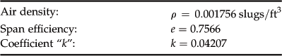
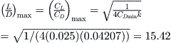

Figure 20-8 shows the drag polar and L/D graph for this airplane. A summary of results is provided in Table 20-4.
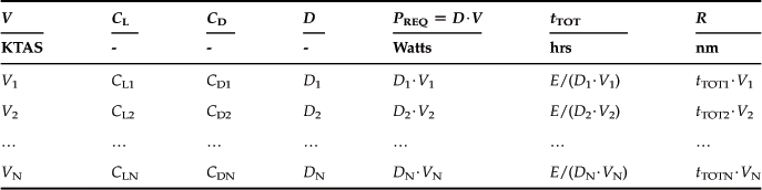
TABLE 20-4
| Method | Range, nm |
| "Dumbed down" method | 698 |
| Method 1: constant airspeed/altitude cruise | 694 |
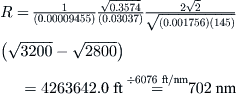
| Method 2: constant attitude/altitude cruise | 702 |
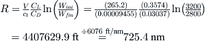
| Method 3: constant airspeed/attitude cruise | 725 |
| Method 4: range at max L/D airspeed (Example 20-6) | 951 |
20.2.6 Determining Fuel Required for a Mission
Sometimes it is necessary to determine the amount of fuel required for a mission. This section determines the fuel required to fly a known distance, assuming the airplane’s weight at the beginning of the cruise segment is known.
Range Profile 1: Constant Airspeed/Altitude Cruise
This condition is the norm for commercial and freight aircraft, as they are directed by air traffic controllers (ATC) to maintain uniform airspeed and altitude to simplify management of air traffic. Unfortunately, the resulting expression is transcendental and must thus be solved iteratively.
![]() (20-14)
(20-14)
Derivation of Equation (20-14)
The Breguet range equation for this condition is given by Equation (20-10):
![]()
![]()
QED
Range Profile 3: Constant Airspeed/Attitude Cruise
This profile is far less common in normal operation of aircraft, but would be used to optimize long range for specialized aircraft.
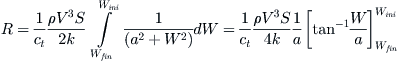
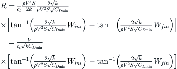
![]() (20-15)
(20-15)
20.2.7 Range Sensitivity Studies
As stated in the introduction to this section, range and endurance are of paramount importance to most aircraft design projects. Many types of aircraft are sold only because of their range or endurance. If the predicted range is not met, the entire development project may be compromised. For this reason, it is imperative to assess how sensitive the design will be to deviations from standard operational parameters. For instance, consider a project in which the empty weight ends up being higher than initially expected. This, inevitably, cuts into the fuel quantity that can be carried for the design mission. A sensitivity study can help expose a possible weakness in the design early enough to justify modifications that remedy the situation.
The following examples use the methods presented in this section. For simplicity they do not account for the range accrued during climb or descent. As usual, a sensitivity study usually implies that specific variables are fixed while allowing a target parameter of interest to vary.
Empty Weight Sensitivity
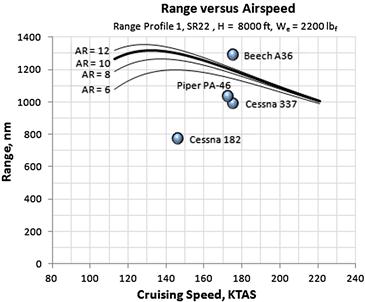
The empty weight sensitivity shows the effect of deviations in empty weight on the range of the airplane (see Figure 20-9). Here, assume the target empty weight to amount to 2200 lbf. If the production aircraft ends up being 300 lbf heavier than anticipated, the maximum range drops from about 1315 nm to about 771 nm for the particular loading (which here consists of two 200 lbf individuals and 50 lbf of baggage).

It is helpful to plot the capability of the competition on the weight sensitivity graph. This will help relay the comparative capability of the new design.
Drag Sensitivity
The drag sensitivity shows the effect of deviations in drag coefficient on the range of the airplane (see Figure 20-10). Here, the target empty weight is assumed 2200 lbf. If the production aircraft generates 20 drag counts above expected value, the baseline range of 1315 nm drops to 1240nm and 1180 nm if it generates 40 additional drag counts. The additional drag can stem from a number of sources. For instance, larger than expected flow separation regions during cruise (poor wing fairing design, poor geometric quality), non-materialization of NLF (turbulent boundary layer in regions where NLF is expected), protrusions such as antennas and entry steps, cooling drag, CRUD, and so on.

Aspect Ratio Sensitivity
The aspect ratio sensitivity reveals the effect of the wing AR on the range of the airplane (see Figure 20-11). Here, the target AR of 10 yields a baseline range of 1315 nm. Reducing this to, say, 6 results in a drop of 115 nm to 1200 nm.
The primary advantage of AR is reduction in lift induced drag. Most of this is realized at lower dynamic pressures, when the airplane must fly at higher AOAs.
20.3 Specific Range
20.3.1 Definitions
Specific range (SR) is the distance an airplane can fly on a given amount of fuel. This quantity is important when comparing the efficiency of different aircraft types or different airspeeds for an individual aircraft, for instance, when determining at which airspeed a particular airplane is the most efficient.
![]() (20-16)
(20-16)
Specific range is analogous to the term gas mileage as used for cars; the primary difference is that when used for airplanes one usually specifies fuel quantity in terms of lbf rather than gallons. Knowing the range flown and weight of the fuel consumed during that segment, we can calculate the average SR from the following expression:
![]() (20-17)
(20-17)
We can also compute the instantaneous SR as follows:
![]() (20-18)
(20-18)
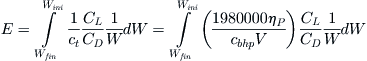
20.3.2 CAFE Foundation Challenge
In 2010 the CAFE Foundation announced a competition aimed at encouraging the aviation industry to go “green”. To lead the way, the $1.65M NASA-funded CAFE Green Flight Challenge is a flight competition for quiet, practical, “green” aircraft that took place July 11–17, 2011, at the CAFE Foundation Flight Test Center at Charles M. Schulz Sonoma County Airport in Santa Rosa, California. The winning aircraft (Team Pipistrel-USA.com), a four-seat electric-powered version of the Taurus G4, flew 192 statute-miles non-stop, achieving an astounding mileage of 403.5 passenger·mi/gal. This amounts to one person being able to travel 403.5 mi (351 nm) on one gallon of fuel (or two persons travelling 202 mi per gallon of fuel). It demonstrated the possibilities offered by electric aircraft of the future.
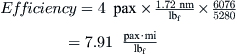
The goal of the challenge was to achieve 200 pax·mi/gal. In essence, this requires the following efficiency:
![]()
For the two people on board this corresponds to a SR of:
![]()
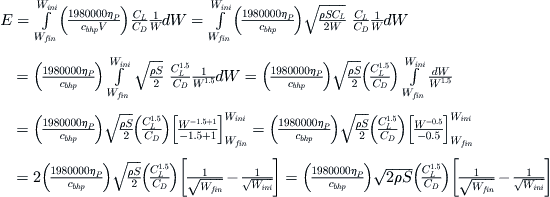
This value is called “specific range”. In terms of the Brequet flight profile 3, the range per pound of fuel consumed amounts to:
![]()
EXAMPLE 20-9
Estimate the efficiency of the SR22 (see Figure 20-12) if, per its POH, the specific range at 75% power at 8000 ft is 10.3 nm/gal.
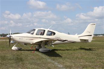
Solution
Convert the specific range to nm/lbf of fuel:
![]()
Therefore, the efficiency can be calculated as follows:
20.4 Fundamental Relations for Endurance Analysis
The following mathematical expressions can be used to estimate the endurance with the cited restrictions. An inspection of the resulting equations demonstrates a certain commonality between all. In other words, in order to achieve a long endurance capability the airplane must be designed with the following features in mind:
(1) It must have a high operational L/D ratio. In other words, it must feature as low drag as possible.
(2) It must have a low specific fuel consumption (or low thrust specific fuel consumption).
(3) If driven by a propeller it must feature the highest possible propeller efficiency and operate at a low altitude (high ρ).
Formulation for the estimation of endurance will now be developed assuming the same profiles used for the development of range.
20.4.1 Endurance Profile 1: Constant Airspeed/Constant Altitude Cruise
Refer to Section 20.2.2, Range profile 1: constant airspeed/constant altitude cruise and Figure 20-5 for more details on this cruise profile. This result is valid only for the simplified drag model.
![]() (20-19)
(20-19)
Derivation of Equation (20-19)
In all three cases, the thrust specific fuel consumption, ct, is constant. Additionally for this case, the airspeed, V, is also constant. However, CL/CD is not. Therefore, we write Equation (20-7), introducing the simplified drag model as follows:
Expanding by inserting the expressions for the lift coefficient we get:
Manipulate algebraically to get:

Let’s define the constant a as follows:
![]()
Then insert and solve:

QED
20.4.2 Endurance Profile 2: Constant Attitude/Altitude Cruise
Refer to Section 20.2.3, Range profile 2: constant altitude/constant attitude cruise and Figure 20-5 for more details on this cruise profile. Both following results are valid regardless of drag model choice.
For a jet:
![]() (20-20)
(20-20)
Note that a special version of this expression extends to propeller aircraft due to the fact that the thrust specific fuel consumption is dependent on the airspeed (see Section 20.1.7, Notes on SFC and TSFC).
For a propeller:
![]() (20-21)
(20-21)
The constant 1980000 allows the SFC, represented by the variable c, to be entered in terms of lbf of fuel per hour per BHP (i.e. lbf/hr/BHP), but this is conveniently the most common presentation of this important parameter the designer will come across.
Derivation of Equation (20-20)
The derivation is straightforward. Since the attitude is constant, move CL/CD outside the integral and integrate:

QED
20.4.3 Endurance Profile 3: Constant Airspeed/Attitude Cruise
Refer to Section 20.2.4, Range profile 3: constant airspeed/constant attitude cruise and Figure 20-7 for more details on this cruise profile. Valid for both jets and propeller-driven aircraft and independent of the drag model:
![]() (20-22)
(20-22)
Derivation of Equation (20-22)
Again, the derivation is straight forward. Since the attitude is constant, move CL/CD outside the integral and integrate:

QED
EXAMPLE 20-10
The light airplane of EXAMPLE 20-1 starts its cruise segment at 135 KCAS at 10,000 ft when it weighs 3200 lbs. After cruising for a period of time at that altitude it is noticed it now weighs 2800 lbs. The following additional data is given:
| Wing area | S = 145 ft² |
| Aspect ratio | AR = 10 |
| Minimum drag coefficient | CDmin = 0.025 |
| Average fuel burn | 15 gallons/hr |
| Average BHP | 150 BHP |
| Propeller efficiency | ηp = 0.85 |
Compute the endurance of this airplane using the first profile.
Note that this is EXAMPLE 20-5 from the range portion solved for endurance.

20.5 Analysis of Mission Profile
Now that the formulation to estimate range and endurance has been developed, it is appropriate to introduce the fundamentals of mission analysis. A mission analysis is the investigation of an entire flight of an airplane, from engine start to shut-down. Generally, such analysis breaks the mission into several distinct segments, which allows for a simpler analysis of each and important properties of the airplane, such as weight, airspeed, and others to be determined more easily.
Any serious mission planning must account for (a) fuel required to complete the mission and (b) additional fuel to allow the airplane to be diverted from the destination airport to some alternative airport should inclement weather compromise a safe landing. The additional fuel is called reserve fuel. The preceding sections have not accounted for this fuel, but rather assumed this as a part of the empty weight (which it is not) or simply ignored it. Any range or endurance analysis should accommodate reserve fuel in the final weight (Wfin) – naturally, reducing the total fuel available for the design mission. The reserve fuel must be sufficient to allow the airplane to climb to a new cruise altitude after an attempted and missed approach for landing, and continue flying to an alternative airport that may be as far as 100 or 200 nm from the original destination. There are generally two operational cruise missions that designers of civilian aircraft should be aware of: IFR and NBAA missions. These will be discussed later in this section. First, fundamentals of mission analysis will be presented.
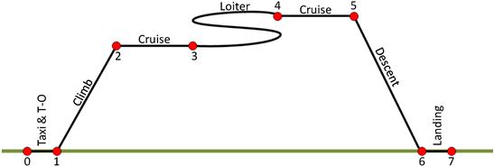
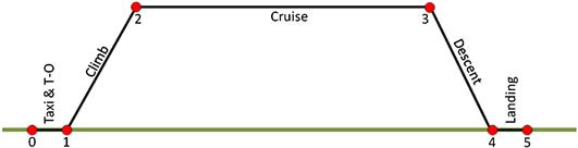
20.5.1 Basics of Mission Profile Analysis
Clearly, the weight of the fuel required to complete the design mission is of paramount importance and accurate range estimation must account for all the fuel that will be consumed. Consider a scenario in which the mission, from engine start until engine shut-down, consists of the segments shown in Figure 20-13. Each segment is denoted as a line drawn between two points, or nodes. Each node is numbered from 0 to 7. Of course the mission may be more complicated than shown here; however, it can also be far simpler. At any rate, the important element is to recognize that as the airplane covers each segment, assuming it uses fossil fuels, its weight is reduced. This way, the weight of the airplane at Node 1 is less than at Node 0. Similarly, after climbing to its cruise altitude, denoted by Node 2, its weight is less than after T-O at Node 1, and so on. Clearly, the difference between each subsequent node is the amount of fuel consumed during the segment, although it may also include the weight of parachutists or external stores.
In order to analyze the entire mission, we observe that (note the difference WO {“O” for gross weight} versus W0 {“zero” for Node 0}, which indicates that the airplane does not always take off at gross weight):
And so forth. If we know the average fuel consumption in fuel weight/unit time during the segment and the time it takes to complete the segment we can always estimate the ratio as follows. Note that if the fuel consumption (or “fuel flow”) is in terms of lbf/hr, the time would have to be in terms of hours:
![]() (20-25)
(20-25)
where
Naturally, if the airplane features items that can be jettisoned, such as military ordnance or fuel tanks, or fertilizer from agricultural aircraft, or even fuel during an emergency fuel dump operation, a different set of relations would have to be established.
Weight ratios for selected segments
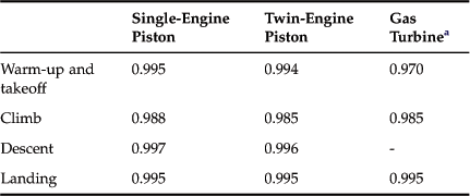
Since the cruise segment often remains the unknown variable in mission analyses (see EXAMPLE 20-12), the weight ratios associated with the other segments must be known. As an example, some of the segments shown in Figure 20-13 lend themselves to a generalized approach: for instance the engine start, warm-up, takeoff, climb, and landing. It is a reasonable assumption that the ratios for these phases remain constant for any particular class of aircraft. In this context, Table 20-6 it may be helpful for filling in some of the gaps in the mission analysis.
20.5.2 Methodology for Mission Analysis
An example of a simple mission is shown in Figure 20-14. It consists of segments that entail engine start, warm-up, run-up, taxi into T-O position, the T-O, climb to cruise altitude, cruise, descent, landing, and finally taxi and parking. In the interests of clarity, the segments have been combined and are identified at each intersection by the six nodes. Each node has a weight associated with it, denoted by W0, W1, …, W5. Then, the mission is analyzed by determining the weight (and therefore fuel consumed) at each node.

As an example of the analysis methodology, consider a scenario in which we have to determine the fuel available for cruise (cruise range); this is the fraction W3/W2 in Figure 20-14. In most cases, the engine start-up weight, W0, and mission fuel weight, Wfm, are known. Assume it has been estimated (for instance using historical data or knowledge of engine fuel consumption) that the engine start-up, warm-up, and taxi to T-O position consumes fuel so at Node 1 the airplane weighs 99% of W0. In this case it is possible to write the weight at Node 1 as follows:
![]()
Similarly, assume that during the climb to the cruise altitude the airplane consumes fuel such it weighs 93% of the weight at Node 1. This can be based off of the weight at Node 1 as follows:
![]()
In effect, this would allow the weight at Node 2 to be determined based on the initial weight, W0, as shown below:
![]()
This simply means that when the airplane reaches its cruise altitude, it weighs 92.07% of its engine start-up weight. In fact, the entire mission can be represented as the product of the segment weight ratios:
![]()
This representation boils the problem of determining the amount of fuel available for cruise (represented by W3/W2) down to determining the other weight ratios and using them to estimate the desired ratio.
To see how this is accomplished, assume that we have determined that the weight at the point of touch-down (Node 4) is 96% of the weight at cruise let-down (Node 3). Also, assume that at the time of engine shut-down (Node 5), the weight is 99% of the weight at Node 4. If we assume we run out of the mission fuel at Node 5, we can write the weight at Node 5 as follows:
![]()
where Wfm = total mission fuel weight (known).
This allows the mission weight ratio to be rewritten as follows:
![]()
Inserting known ratios leads to:
![]()
This allows the weight ratio at the start and end of cruise to be written as show below:
![]()
Using the value of W2 already determined above and simple algebra, the amount of fuel weight available for the cruise portion amounts to:
![]()
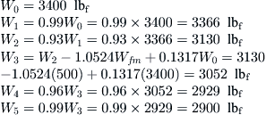
One important observation is that the fuel required to just get the airplane to cruising altitude and return to base (no actual cruise range) is determined by setting the difference W2 − W3 = 0 and solving for Wfm. The resulting minimum fuel amounts to 0.1251W0, or 12.5% of gross weight. If this represented a real aircraft, it would be placed at a significant competitive disadvantage. Thus, if the gross weight of the airplane is 3400 lbf and it has 500 lbf of fuel on board intended for the mission, it will have 1.0524 × 500 – 0.1317 × 3400 = 78.4 lbf of fuel available for the cruise range. The fuel for the entire mission can be broken down as follows:
EXAMPLE 20-11
A small single-engine aircraft is being designed for the mission of Figure 20-13 and it has been established that it consumes 10 lbf of fuel during Segment 0-1. During climb, which starts at sea level, the average fuel burn is 15 gallons per hour and the average rate of climb is 1000 fpm. Determine the weight ratios for the first two segments (taxi & T-O and climb) if its mission cruise altitude is 15,000ft. A gallon of fuel weighs 6 lbf. If its start-up weight is 3400 lbf, what is its weight at Node 2?
EXAMPLE 20-12
The aircraft of EXAMPLE 20-11 is being evaluated based on the mission of Figure 20-13 for fuel requirements between Nodes 2 and 5 assuming all fuel is exhausted at Node 7 and the total fuel weight ratio is 0.15. The following weight ratios have been estimated:
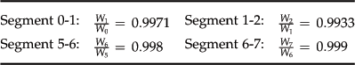
Determine the fuel remaining to complete segments 2-5.
Solution
If we assume all the fuel to be consumed at Node 7, it follows that the total weight ratio between Nodes 0 and 7 will be (noting that a fuel weight ratio of 0.15 means 0.15 × W0):
![]()
We can write the change in weight along the mission shown in Figure 20-13 as follows:
![]()
The expression reveals that only the ratio ![]() is not yet known. We will now solve the above expression for this ratio:
is not yet known. We will now solve the above expression for this ratio:
![]()
We have already calculated the weight of the airplane at Node 2 in EXAMPLE 20-11. Using that result we can easily estimate the weight of the aircraft at Node 5:
![]()
Therefore, the fuel required between Nodes 2 and 5 is 3367 − 2898 = 469 lbf or just over 78 gallons.
20.5.3 Special Range Mission 1: IFR Cruise Mission
GA aircraft intended for operation under Instrument Flight Rules (IFR) must carry fuel in compliance with 14 CFR Part 91, § 91.167, Fuel Requirements for Flight in IFR Conditions. The regulation is intended to prevent accidents due to fuel starvation or fuel mismanagement, but such accidents, in spite of the regulation, remain fairly common, with 75 such accidents in 2008 and 74 in 2009 in the US alone [8]. GA aircraft operated in IFR conditions must carry fuel as stipulated below:
The paragraph requires the operator of the aircraft to carry enough fuel to complete the flight to the initial airport, then fly from that airport to the alternative airport (if one is required) and, then fly for 45 minutes (30 minutes for helicopters) at normal cruising speed [9]. In short, it is fuel to the destination plus fuel to the alternative plus fuel for 45 minutes of additional flying. It is important for the designer to be mindful of such regulatory “curveballs” so that the range (or size of fuel tanks) won’t be incorrectly estimated.
A schematic of an IFR flight profile is shown in Figure 20-15. The term STD IFR APP stands for Standard IFR Approach. Even though such flight planning is the responsibility of the operator, it is only prudent the designer should prepare range estimation for comparison with other aircraft by assuming a 100 or 200 nm diverted flight to an alternative, depending on the size of the aircraft. This will shed a much clearer light on the utility of the new design.

20.5.4 Special Range Mission 2: NBAA Cruise Mission
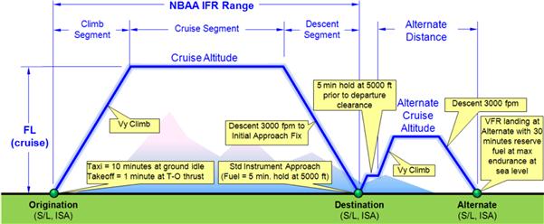
The National Business Aviation Association (NBAA) is an organization of people who try to promote and expand the use of General Aviation aircraft for business purposes globally [10]. It was founded in 1947 and has its headquarters in Washington DC. According to its Statement of Purpose, the organization represents more than 8000 companies and organizes the world’s largest aviation trades show; the NBAA Annual Meeting & Convention. When it comes to the concept of range, NBAA has promoted a special range profile that carries its name. A schematic of this profile is provided in Figure 20-16. This profile is typically used in the marketing of business aircraft.
20.5.5 Payload-Range Sensitivity Study
It is helpful, even when not mandated, to conduct a payload-range sensitivity study to help evaluate how payload affects the range of the aircraft. Most small aircraft have issues with the combination of fuel and occupant loading. This manifests itself as an inability to take off simultaneously with the fuel tanks and seats filled without busting the max gross weight limit. Thus, most small aircraft have to limit fuel weight when flying with full occupancy and this can reduce their range significantly.
Figure 20-17 illustrates the problem using a hypothetical single-pilot-operated ten-seat turboprop commuter design of a maximum design gross weight of 7500 lbf. Assume the airplane is designed to carry as much as 2000 lbf of Jet A-1, which gives it a range of 1100 nm. This means that no matter the combination of fuel, passengers, and baggage, the airplane shall not exceed 7500 lbf at the start of the T-O run. Furthermore, assume that based on historical data it is expected an empty weight ratio of 0.6 can be achieved. This corresponds to an empty weight of 4500 lbf and useful load of 7500 − 4500 = 3000 lbf. If each occupant can weigh as much as 200 lbf, including baggage, it is easy to see that, with 10 people onboard, the airplane will weigh 4500 + 10 × 200 = 6500 lbf; this corresponds to a payload of nine people (the pilot is not a part of the payload) or 1800 lbf. As a consequence the pilot can only add 1000 lbf of fuel and, thus, will not achieve the full tank range of 1100 nm. Here, for simplicity, it is assumed the aircraft can achieve the hypothetical range of 0.55 nm per lbf of fuel.
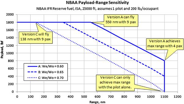
Results for other payloads are presented in Table 20-7 (and graphically in Figure 20-17). It is intended to help with the preparation of such sensitivity graphs. It displays not only how range is affected by payload, but also how detrimental it may be if the desired empty weight ratio is not met. Payload-range sensitivity studies are very helpful when evaluating new aircraft designs and clearly highlights the importance of achieving the design empty-weight ratio.
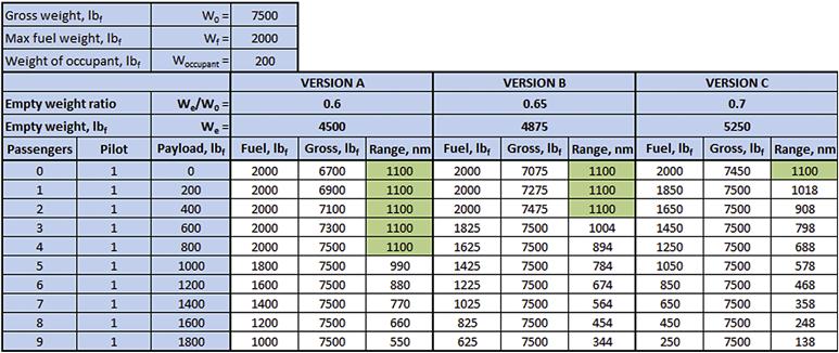
Table 20-7 presents the payload-range sensitivity for three empty weight ratios; 0.60, 0.65, and 0.70, designated as Versions A, B, and C, respectively. Thus, Version A can carry four passengers and pilot 1100 nm, while it can only achieve 550 nm with nine passengers onboard. However, if the empty weight ratio of 0.60 is not met and, say, it ends up being 0.65 (Version B), the airplane will be much less competitive as it can only fly 1100 nm with two passengers onboard. If the empty weight ratio ends up being 0.70 (Version C), the market prospects of the resulting aircraft may in fact be catastrophic. This highlights its sensitivity to deviations from the target empty weight ratio.
Exercises
(1) (a) A twin-piston-engine aircraft is being designed for the mission of Figure 20-18 and it has been established that it consumes 30 lbf of fuel during Segment 0-1. During climb, which starts at sea level, the average fuel burn is 44 gallons per hour and the average rate of climb is 1600 fpm. Determine the weight ratios for the taxi & T-O and climb segments if its design mission cruise altitude is 20,000 ft. A gallon of fuel weighs 6 lbf. If its start-up weight is 5500 lbf, what is its weight at Node 2?
(b) Using the mission of Figure 20-18 estimate the fuel requirements between Nodes 2 and 3 assuming all fuel is exhausted at Node 5 and the total fuel weight ratio is 0.18. Use the weight ratios of Table 20-6 for descent and landing.
(2) You have been asked to design a single-engine, turbofan-powered research aircraft that, on a no-wind standard day, is capable of an 800 nm loiter range. The loitering segment will begin at an initial altitude of 20,000 ft and requires a constant airspeed of 250 KTAS to be maintained. The research equipment on board must be calibrated at the beginning of the segment, after which the autopilot is programmed to maintain constant attitude of the aircraft with respect to the ground. The SFC of the turbofan is 0.6 lbf/hr/lbf, wing area is 350 ft², and the weight at the start of cruise is 15,000 lbf. The average fuel consumption of the engine during the loitering segment is 115 gallons/hr of Jet-A. If you are considering a configuration featuring a straight tapered wing with an AR of 10, estimate (a) the highest value the minimum drag coefficient, CDmin, can take and still meet the range requirement. (b) Also, estimate thrust required at the start of cruise. Assume the simplified drag model applies.
Answer: (a) CDmin = 0.0295, (b) T = 1403 lbf.

References
1. Perkins CD, Hage RE. Airplane Performance, Stability, and Control. John Wiley & Sons 1949.
2. Torenbeek E. Synthesis of Subsonic Aircraft Design. 3rd edn Delft University Press 1986.
3. Nicolai L. Fundamentals of Aircraft Design. 2nd edn 1984.
4. Roskam J, Lan Chuan-Tau Edward. Airplane Aerodynamics and Performance. DARcorporation 1997.
5. Hale FJ. Aircraft Performance, Selection, and Design. John Wiley & Sons 1984; 137–138.
6. Anderson Jr JD. Aircraft Performance & Design. 1st edn McGraw-Hill 1998.
7. Raymer D. Aircraft Design: A Conceptual Approach. AIAA Education Series 1996.
8. The Nall Report 2010, Air Safety Foundation, p. 17.
9. InFO 08004, Federal Aviation Administration, 02/07/2008.
10. In: http://www.nbaa.org/about/.