
Atmospheric Modeling
A.1 Introduction
A number of organizations and scientists have developed sophisticated models of the atmosphere that allow atmospheric properties at different altitudes to be determined. As an example, the National Oceanic and Atmospheric Administration (NOAA) has developed one of the best known of these, the U.S. Standard Atmosphere 1976 [1]. However, far more sophisticated models than that have been developed. One such model is the NRLMSISE-00 (Naval Research Laboratory Mass Spectrometer and Incoherent Scatter, where E means from surface of the Earth to the Exosphere). This model requests input data in the form of year, day, time of day, altitude, geodetic latitude and longitude, and many others. It returns information such as temperature, mass density, and molecular densities of oxygen (O2), nitrogen (N2), mono-atomic oxygen (O) and nitrogen (N), argon (Ar), and hydrogen (H). These can be used to estimate other properties, such as specific gas constant (typically denoted by R), pressure, and the ratio of specific heats (typically denoted by γ). Among numerous applications, this model is used to predict the orbital decay of satellites due to atmospheric drag and to study the effect of atmospheric gravity waves. An example of output of temperature and density from this atmospheric model is shown in Figure A-1. The figure shows the two gas states up to an altitude of 500 km, well beyond the so-called von Kárman line, which is considered the edge of the atmosphere, as the point where a vehicle would have to fly faster than its orbital escape speed to generate a dynamic pressure large enough to provide aerodynamic lift.
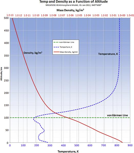
FIGURE A-1 An output from the NRLMSISE-00 atmospheric model showing the variation of temperature and mass density as a function of altitude ranging from S-L to 500 km. The von Kárman Line is considered the “boundary between Earth’s atmosphere and outer space.” It is the altitude where aerodynamic forces can no longer provide support to maintain altitude, so vehicles must be in orbit in order to do so.
In this text, all atmospheric data is based on the US Standard Atmosphere 1976, unless otherwise specified. This is done because it can be conveniently represented using simple formulation. Additionally, examples in this book take place in the troposphere, below 36,089 ft (see Figure A-2).
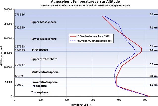
FIGURE A-2 A comparison of temperature changes with altitude up to 85 km, using the US Standard Atmosphere 1976 and NRLMSISE-00 atmospheric models. The former represents standard conditions, whereas the latter is at a geodesic location N45° W80° on January 1st, 2012.
A.1.1 General Information About the Atmosphere
An atmosphere is the mixture of gases surrounding a celestial object (i.e. planet) whose gravitational field is strong enough to prevent its molecules from escaping. In particular, the atmosphere refers to the gaseous envelope of the Earth.
Formation of
The current mixture of gases in the air is thought to have taken some 4.5 billion years to evolve. The early atmosphere is believed to have consisted of volcanic gases alone. Since gases from erupting volcanoes today are mostly a mixture of water vapor (H2O), carbon dioxide (CO2), sulfur dioxide (SO2), and nitrogen (N) it is postulated that this was probably the composition of the early atmosphere as well. It follows that a number of chemical processes must have preceded the mixture making the atmosphere of our time.
One of those processes is thought to have been condensation, which was a natural consequence of the cooling of the earth’s crust and early atmosphere. This condensation is thought to have slowly but surely filled valleys in the barren landscape, forming the earliest oceans. Some CO2 would have reacted with the rocks of the earth’s crust to form carbonate minerals, while some would have dissolved in the new rising oceans. Later, as primitive life capable of photosynthesis evolved in the oceans, new marine organisms began producing oxygen. Almost all the free oxygen in the air today is attributed to this process; by photosynthetic combination of CO2 with water.
About 570 million years ago, the oxygen content of the atmosphere and oceans became high enough to permit marine life capable of respiration; 170 million years later, the atmosphere would have contained enough oxygen for air-breathing animals to emerge from the seas.
A.1.2 Chemical Composition of Standard Air
Research shows the chemical composition of the atmosphere is practically independent of altitude from ground level to at least 88 km (55 mi). The continuous stirring produced by atmospheric currents counteracts the tendency of the heavier gases to settle below the lighter ones. In the lower atmosphere ozone is present in extremely low concentrations. The layer of atmosphere from 19 to 48 km (12 to 30 mi) up contains more ozone, produced by the action of ultraviolet radiation from the sun. Even in this layer, however, the percentage of ozone is only 0.001 by volume. Atmospheric disturbances and downdrafts carry varying amounts of this ozone to the surface of the earth. Human activity adds to ozone in the lower atmosphere, where it becomes a pollutant that can cause extensive crop damage. Table A-1 lists the chemical composition of the atmosphere.

A.1.3 Layer Classification of the Atmosphere
The atmosphere is generally divided into several layers based on some specific characteristics (see Table A-2). The troposphere extends from the ground to some 11–16 km (6.8–10 mi) and this is where most clouds occur and weather (winds and precipitation) are most active. It transitions into the next layer; the stratosphere, through a thin region called the tropopause. The bulk of the atmosphere is found within these two lowest layers. Above the stratosphere is the mesosphere, which is characterized by a decrease in temperature with altitude. Research of propagation and reflection of radio waves starting at an altitude of 80 km (50 mi) to some 640 km (400 mi) indicates that ultraviolet radiation, X-rays, and showers of electrons from the sun ionize this layer of the atmosphere, causing it to conduct electricity and reflect radio waves of certain frequencies back to earth. For this reason, it is called the ionosphere. It is also termed the thermosphere, because of the relatively higher temperatures in this layer. Above it is the exosphere, which extends to the outer limit of the atmosphere, at about 9600 km (about 6000 mi). Figure A-2 shows how temperature changes through the lowest layers of the atmosphere. The classification of the atmosphere is based on an average height of the layers.
TABLE A-2
Layer Classification of the Atmosphere
| Name of Layer | Altitude in km | Altitude in Statute Miles |
| Tropospherea | 0–11 km | 0–6.8 sm |
| Tropopause | 11–11.5 km | 6.8–1 sm |
| Stratosphere | 11.5–46 km | 11.5–29 sm |
| Stratopause | 46–51 km | 29–32 sm |
| Mesosphere | 51–85 km | 32–53 sm |
| Ionosphere (Thermosphere) | 85–640 km | 53–400 sm |
| Exosphere | 640–9600 km | 400–6000 sm |
aIn temperate latitudes this is approximately 0–9.7 km (6 mi). The troposphere can extend to 15 km in the tropics.
A.2 Modeling Atmospheric Properties
A.2.1 Atmospheric Ambient Temperature
Let’s start by considering the temperature, T. Change in air temperature with altitude can be approximated using a linear function:
![]() (A-1)
(A-1)
An alternative form of Equation (A-1) is:
![]() (A-2)
(A-2)
where
A.2.2 Atmospheric Pressure and Density for Altitudes below 36,089 ft (11,000 m)
The hydrostatic equilibrium equations allow the pressure, p, and density, ρ, to be calculated as functions of altitude, h, as follows:
Derivation of Equations (A-3) and (A-4)
Begin with the hydrostatic equilibrium equation and divide by the ideal gas relation as shown below:
 (i)
(i)
Differentiate Equation (A-1) (which is T(h)):
![]()
Insert our expression for the temperature:
![]()
Insert standard day coefficients for troposphere:
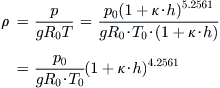
We’d also like to derive an expression for density as a function of altitude. To do this, we start by rewriting Equation (C-6) in terms of density:
![]()
Then, we insert the expressions for temperature and density and expand as follows:
QED
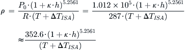
A.2.3 Density of Air Deviations From a Standard Atmosphere
Atmospheric conditions often deviate from models shown above. Such deviations can be handled as reflected below, using the UK system:
![]() (A-5)
(A-5)
where
T = standard day temperature at the given altitude per the International Standard Atmosphere. in °R; at S-L it would be 518.67 °R, at 10,000 ft it would be 483 °R, and so on
ΔTISA = deviation from International Standard Atmosphere in °F or °R
![]() (A-6)
(A-6)
where
T = standard day temperature at the given altitude per the International Standard Atmosphere. in degrees K; at S-L it would be 288.15 K, at 10,000 ft it would be 483 °R, and so on
ΔTISA = deviation from International Standard Atmosphere in °F or °R
For non-standard atmosphere, use a negative sign for colder and a positive sign for warmer than ISA for ΔTISA.
Derivation of Equations (A-5) and (A-6)
Starting with the equation of state we get:
![]()
where T is the standard day temperature in °R at the altitude h, and P0 is the S-L pressure. If working with the UK system, this can be written in a simpler form as follows:
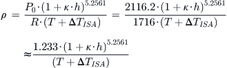
Conversely, if working with the SI system, this can be written as:
QED
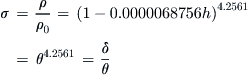
A.2.4 Atmospheric Property Ratios
The pressure, density, and temperature often appear in formulation as fractions of their baseline values. As a consequence, they are identified using special characters and are called pressure ratio, density ratio, and temperature ratio.

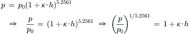
A.2.5 Pressure and Density Altitudes Below 36,089 ft (11,000 m)
Sometimes the pressure or density ratios are known for one reason or another. It is then possible to determine the altitudes to which they correspond. For instance, if the pressure ratio is known, we can calculate the altitude to which it corresponds. The altitude is then called pressure altitude. Similarly, from the density ratio we can determine the density altitude.
Derivation of Equations (A-10) and (A-11)
Begin with Equation (A-3) and solve for the altitude h, through the following algebraic maneuvers:
![]()
Inserting the coefficient κ = −0.0000068756/ft (from Table 16-2) and carrying out the arithmetic yields Equation (A-10). The derivation of Equation (A-11) is identical.
QED
A.2.6 Viscosity
Dynamic or Absolute Viscosity
Viscosity is a measure of a fluid’s internal resistance to deformation and is generally defined as the ratio of the shearing stress to the velocity gradient in the fluid as it flows over a surface. Mathematically this is expressed using the following expression:
![]() (A-12)
(A-12)
where ![]() velocity gradient in a fluid as it moves over a surface
velocity gradient in a fluid as it moves over a surface
The viscosity coefficient we are primarily interested in is that of air. It can be determined using the following empirical expression, which assumes the UK system of units and, therefore, the temperature in °R (Ref. [2], Equation (2.90)):
![]() (A-13)
(A-13)
In the SI system the temperature is given in K and the viscosity can be found from (Ref. [2], Equation (2.91)):
![]() (A-14)
(A-14)
where
Kinematic Viscosity
This is defined as the dynamic viscosity divided by the fluid density:
![]() (A-15)
(A-15)
The units for kinematic viscosity are 1/(ft²·s) in the UK system and 1/(m²·s) in the SI system.
A.2.7 Reynolds Number
The Reynolds number of a fluid is determined from the relationship below:
![]() (A-16)
(A-16)
where
L = reference length (for instance MAC), in ft or m
V = reference airspeed, in ft/s or m/s
ρ = fluid density, in slugs/ft3 or kg/m3
μ = fluid (dynamic) viscosity, in lbf·s/ft² or N·s/m²
A simple expression, valid for the UK system at sea-level conditions only is (V and L are in ft/s and ft, respectively):
![]() (A-17)
(A-17)
A simple expression, valid for the SI system at sea-level conditions only is (V and L are in m/s and m, respectively):
![]() (A-18)
(A-18)
A.2.8 Speed of Sound and Mach Number
The speed of sound is retrieved from the expression below:
![]() (A-19)
(A-19)
![]() (A-20)
(A-20)
where
R = universal gas constant (1716 ft·lbf/slug·°R)
EXAMPLE A-2
Determine the speed of sound at 8500 ft on a standard day using both forms of Equation (C-14).
A.2.9 Atmospheric Modeling
As stated earlier, the properties of the atmosphere above the troposphere are detailed in the document US Standard Atmosphere 1976, published by NOAA,1 NASA,2 and the US Air Force. The formulation in Table A-3 is based on a summary from http://www.atmosculator.com/, which is based on the US Standard Atmosphere 1976. The temperature (in °R), pressure (in lbf/ft²), and density (in slugs/ft3) are plotted in Figure A-3 from S-L to 278,386.
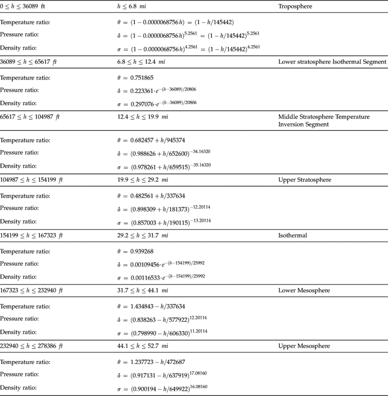
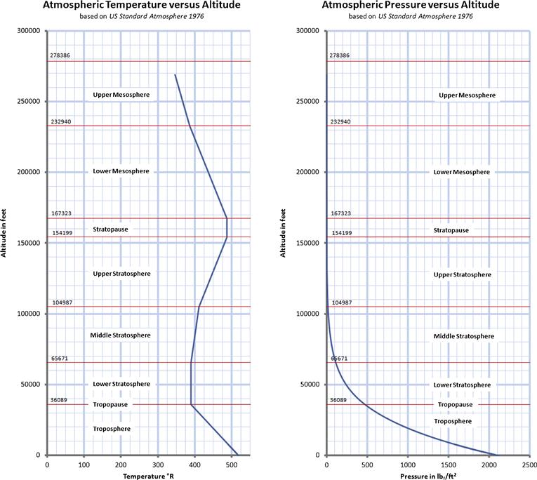
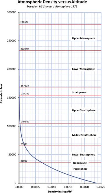
FIGURE A-3 The US Standard Atmosphere 1976 plotted from S-L to 278,386 ft, using the formulation in Section A.2.9, Atmospheric modeling.
A.2.10 COMPUTER CODE A-1: Atmospheric Modeling
The following function, written in Visual Basic for Applications, can be used in Microsoft Excel to determine temperature, pressure, or density at any altitude up to 278,386 ft. To use, insert a VBA module into the spreadsheet and enter the function. Assume we have entered an altitude in cell A1. Then calls are made to it from any other cell by entering a statement like “=AtmosProperty(A1,0).” The rightmost argument (i.e. the “, 0”), called the PropertyID, would cause the function to return the Temperature ratio. If the PropertyID were 10 (i.e. the “, 10”) it would return the temperature, and so on. The allowable values for PropertyID are shown in the comment lines below.
References
1. U.S Standard Atmosphere. National Oceanic and Atmospheric Administration 1976; 1976.
2. Roskam J, Lan Chuan-Tau Edward. Airplane Aerodynamics and Performance. DARcorporation 1997.