13
Concurrent Hashing and Natural Parallelism
13.1 Introduction
In earlier chapters, we studied how to extract parallelism from data structures like queues, stacks, and counters, that seemed to provide few opportunities for parallelism. In this chapter we take the opposite approach. We study concurrent hashing, a problem that seems to be “naturally parallelizable” or, using a more technical term, disjoint–access–parallel, meaning that concurrent method calls are likely to access disjoint locations, implying that there is little need for synchronization.
Hashing is a technique commonly used in sequential Set implementations to ensure that contains(), add(), and remove() calls take constant average time. The concurrent Set implementations studied in Chapter 9 required time linear in the size of the set. In this chapter, we study ways to make hashing concurrent, sometimes using locks and sometimes not. Even though hashing seems naturally parallelizable, devising an effective concurrent hash algorithm is far from trivial.
As in earlier chapters, the Set interface provides the following methods, which return Boolean values:
![]() add(x) adds x to the set. Returns true if x was absent, and false otherwise,
add(x) adds x to the set. Returns true if x was absent, and false otherwise,
![]() remove(x) removes x from the set. Returns true if x was present, and false otherwise, and
remove(x) removes x from the set. Returns true if x was present, and false otherwise, and
![]() contains(x) returns true if x is present, and false otherwise.
contains(x) returns true if x is present, and false otherwise.
When designing set implementations, we need to keep the following principle in mind: we can buy more memory, but we cannot buy more time. Given a choice between an algorithm that runs faster but consumes more memory, and a slower algorithm that consumes less memory, we tend to prefer the faster algorithm (within reason).
A hash set (sometimes called a hash table) is an efficient way to implement a set. A hash set is typically implemented as an array, called the table. Each table entry is a reference to one or more items. A hash function maps items to integers so that distinct items usually map to distinct values. (Java provides each object with a hashCode() method that serves this purpose.) To add, remove, or test an item for membership, apply the hash function to the item (modulo the table size) to identify the table entry associated with that item. (We call this step hashing the item.)
In some hash-based set algorithms, each table entry refers to a single item, an approach known as open addressing. In others, each table entry refers to a set of items, traditionally called a bucket, an approach known as closed addressing.
Any hash set algorithm must deal with collisions: what to do when two distinct items hash to the same table entry. Open-addressing algorithms typically resolve collisions by applying alternative hash functions to test alternative table entries. Closed-addressing algorithms place colliding items in the same bucket, until that bucket becomes too full. In both kinds of algorithms, it is sometimes necessary to resize the table. In open-addressing algorithms, the table may become too full to find alternative table entries, and in closed-addressing algorithms, buckets may become too large to search efficiently.
Anecdotal evidence suggests that in most applications, sets are subject to the following distribution of method calls: 90% contains(), 9% add(), and 1% remove() calls. As a practical matter, sets are more likely to grow than to shrink, so we focus here on extensible hashing in which hash sets only grow (shrinking them is a problem for the exercises).
It is easier to make closed-addressing hash set algorithms parallel, so we consider them first.
13.2 Closed-Address Hash Sets
Pragma 13.2.1
Here and elsewhere, we use the standard Java List<T> interface (in package java.util.List). A List<T> is an ordered collection of T objects, where T is a type. Here, we make use of the following List methods: add(x) appends x to the end of the list, get(i) returns (but does not remove) the item at position i, contains(x) returns true if the list contains x. There are many more.
The List interface can be implemented by a number of classes. Here, it is convenient to use the ArrayList class.
We start by defining a base hash set implementation common to all the concurrent closed-addressing hash sets we consider here. The BaseHashSet<T> class is an abstract class, that is, it does not implement all its methods. Later, we look at three alternative synchronization techniques: one using a single coarse-grained lock, one using a fixed-size array of locks, and one using a resizable array of locks. Fig. 13.1 shows the base hash set’s fields and constructor. The table[] field is an array of buckets, each of which is a set implemented as a list (Line 2). We use ArrayList<T> lists for convenience, supporting the standard sequential add(), remove(), and contains() methods. The setSize field is the number of items in the table (Line 3). We sometimes refer to the length of the table[] array, that is, the number of buckets in it, as its capacity.
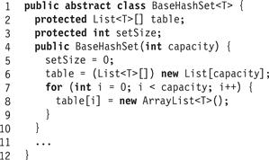
Figure 13.1 BaseHashSet<T> class: fields and constructor.
The BaseHashSet<T> class does not implement the following abstract methods: acquire(x) acquires the locks necessary to manipulate item x, release(x) releases them, policy() decides whether to resize the set, and resize() doubles the capacity of the table[] array. The acquire(x) method must be reentrant (Chapter 8, Section 8.4), meaning that if a thread that has already called acquire(x) makes the same call, then it will proceed without deadlocking with itself.
Fig. 13.2 shows the contains(x) and add(x) methods of the BaseHashSet<T> class. Each method first calls acquire(x) to perform the necessary synchronization, then enters a try block whose finally block calls release(x). The contains(x) method simply tests whether x is present in the associated bucket (Line 17), while add(x) adds x to the list if it is not already present (Line 26).
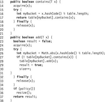
Figure 13.2 BaseHashSet<T> class: the contains() and add() methods hash the item to choose a bucket.
How big should the bucket array be to ensure that method calls take constant expected time? Consider an add(x) call. The first step, hashing x, takes constant time. The second step, adding the item to the bucket, requires traversing a linked list. This traversal takes constant expected time only if the lists have constant expected length, so the table capacity should be proportional to the number of items in the table. This number may vary unpredictably over time, so to ensure that method call times remain (more-or-less) constant, we must resize the table every now and then to ensure that list lengths remain (more-or-less) constant.
We still need to decide when to resize the hash set, and how the resize() method synchronizes with the others. There are many reasonable alternatives. For closed-addressing algorithms, one simple strategy is to resize the set when the average bucket size exceeds a fixed threshold. An alternative policy employs two fixed integer quantities: the bucket threshold and the global threshold.
![]() If more than, say, 1/4 of the buckets exceed the bucket threshold, then double the table capacity, or
If more than, say, 1/4 of the buckets exceed the bucket threshold, then double the table capacity, or
![]() If any single bucket exceeds the global threshold, then double the table capacity.
If any single bucket exceeds the global threshold, then double the table capacity.
Both these strategies work well in practice, as do others. Open-addressing algorithms are slightly more complicated, and are discussed later.
13.2.1 A Coarse-Grained Hash Set
Fig. 13.3 shows the CoarseHashSet<T> class’s fields, constructor, acquire(x), and release(x) methods. The constructor first initializes its superclass (Line 4). Synchronization is provided by a single reentrant lock (Line 2), acquired by acquire(x) (Line 8) and released by release(x) (Line 11).
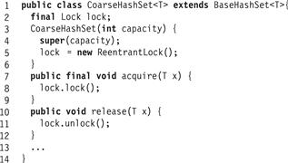
Figure 13.3 CoarseHashSet<T> class: fields, constructor, acquire(), and release() methods.
Fig. 13.4 shows the CoarseHashSet<T> class’s policy() and resize() methods. We use a simple policy: we resize when the average bucket length exceeds 4 (Line 16). The resize() method locks the set (Line 20), and checks that no other thread has resized the table in the meantime (Line 23). It then allocates and initializes a new table with double the capacity (Lines 25–29) and transfers items from the old to the new buckets (Lines 30–34). Finally, it unlocks the set (Line 36).
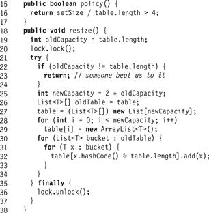
Figure 13.4 CoarseHashSet<T> class: the policy() and resize() methods.
13.2.2 A Striped Hash Set
Like the coarse-grained list studied in Chapter 9, the coarse-grained hash set shown in the last section is easy to understand and easy to implement. Unfortunately, it is also a sequential bottleneck. Method calls take effect in a one-at-a-time order, even when there is no logical reason for them to do so.
We now present a closed address hash table with greater parallelism and less lock contention. Instead of using a single lock to synchronize the entire set, we split the set into independently synchronized pieces. We introduce a technique called lock striping, which will be useful for other data structures as well. Fig. 13.5 shows the fields and constructor for the StripedHashSet<T> class. The set is initialized with an array locks[] of L locks, and an array table[] of N = L buckets, where each bucket is an unsynchronized List<T>. Although these arrays are initially of the same capacity, table[] will grow when the set is resized, but lock[] will not. Every now and then, we double the table capacity N without changing the lock array size L, so that lock i eventually protects each table entry j, where j = i (mod L). The acquire(x) and release(x) methods use x’s hash code to pick which lock to acquire or release. An example illustrating how a StripedHashSet<T> is resized appears in Fig. 13.6.
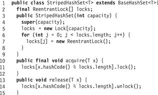
Figure 13.5 StripedHashSet<T> class: fields, constructor, acquire(), and release() methods.
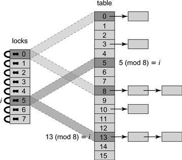
Figure 13.6 Resizing a StripedHashSet lock-based hash table. As the table grows, the striping is adjusted to ensure that each lock covers 2N/L entries. In the figure above, N = 16 and L = 8. When N is doubled from 8 to 16, the memory is striped so that lock i = 5 for example covers both locations that are equal to 5 modulo L.
There are two reasons not to grow the lock array every time we grow the table:
![]() Associating a lock with every table entry could consume too much space, especially when tables are large and contention is low.
Associating a lock with every table entry could consume too much space, especially when tables are large and contention is low.
![]() While resizing the table is straightforward, resizing the lock array (while in use) is more complex, as discussed in Section 13.2.3.
While resizing the table is straightforward, resizing the lock array (while in use) is more complex, as discussed in Section 13.2.3.
Resizing a StripedHashSet (Fig. 13.7) is almost identical to resizing a CoarseHashSet. One difference is that resize() acquires the locks in lock[] in ascending order (Lines 18–20). It cannot deadlock with a contains(), add(), or remove() call because these methods acquire only a single lock. A resize() call cannot deadlock with another resize() call because both calls start without holding any locks, and acquire the locks in the same order. What if two or more threads try to resize at the same time? As in the CoarseHashSet<T>, when a thread starts to resize the table, it records the current table capacity. If, after it has acquired all the locks, it discovers that some other thread has changed the table capacity (Line 23), then it releases the locks and gives up. (It could just double the table size anyway, since it already holds all the locks.)
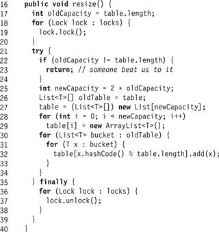
Figure 13.7 StripedHashSet<T> class: to resize the set, lock each lock in order, then check that no other thread has resized the table in the meantime.
Otherwise, it creates a new table[] array with twice the capacity (Line 25), and transfer items from the old table to the new (Line 30). Finally, it releases the locks (Line 36). Because the initializeFrom() method calls add(), it may trigger nested calls to resize(). We leave it as an exercise to check that nested resizing works correctly in this and later hash set implementations.
To summarize, striped locking permits more concurrency than a single coarse-grained lock because method calls whose items hash to different locks can proceed in parallel. The add(), contains(), and remove() methods take constant expected time, but resize() takes linear time and is a “stop-the-world” operation: it halts all concurrent method calls while it increases the table’s capacity.
13.2.3 A Refinable Hash Set
What if we want to refine the granularity of locking as the table size grows, so that the number of locations in a stripe does not continuously grow? Clearly, if we want to resize the lock array, then we need to rely on another form of synchronization. Resizing is rare, so our principal goal is to devise a way to permit the lock array to be resized without substantially increasing the cost of normal method calls.
Fig. 13.8 shows the fields and constructor for the RefinableHashSet<T> class. To add a higher level of synchronization, we introduce a globally shared owner field that combines a Boolean value with a reference to a thread. Normally, the Boolean value is false, meaning that the set is not in the middle of resizing. While a resizing is in progress, however, the Boolean value is true, and the associated reference indicates the thread that is in charge of resizing. These two values are combined in an AtomicMarkableReference<Thread> to allow them to be modified atomically (see Pragma 9.8.1 in Chapter 9). We use the owner as a mutual exclusion flag between the resize() method and any of the add() methods, so that while resizing, there will be no successful updates, and while updating, there will be no successful resizes. Every add() call must read the owner field. Because resizing is rare, the value of owner should usually be cached.
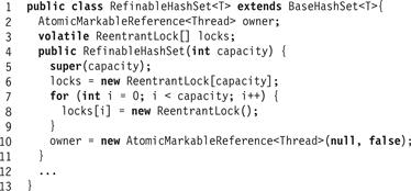
Figure 13.8 RefinableHashSet<T> class: fields and constructor.
Each method locks the bucket for x by calling acquire(x), shown in Fig. 13.9. It spins until no other thread is resizing the set (Lines 19–21), and then reads the lock array (Line 22). It then acquires the item’s lock (Line 24), and checks again, this time while holding the locks (Line 26), to make sure no other thread is resizing, and that no resizing took place between Lines 21 and 26.
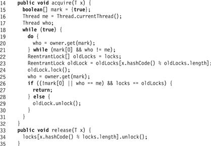
Figure 13.9 RefinableHashSet<T> class: acquire() and release() methods.
If it passes this test, the thread can proceed. Otherwise, the locks it has acquired could be out-of-date because of an ongoing update, so it releases them and starts over. When starting over, it will first spin until the current resize completes (Lines 19–21) before attempting to acquire the locks again. The release(x) method releases the locks acquired by acquire(x).
The resize() method is almost identical to the resize() method for the StripedHashSet class. The one difference appears on Line 46: instead of acquiring all the locks in lock[], the method calls quiesce() (Fig. 13.10) to ensure that no other thread is in the middle of an add(), remove(), or contains() call. The quiesce() method visits each lock and waits until it is unlocked.

Figure 13.10 RefinableHashSet<T> class: resize() method.

Figure 13.11 RefinableHashSet<T> class: quiesce() method.
The acquire() and the resize() methods guarantee mutually exclusive access via the flag principle using the mark field of the owner flag and the table’s locks array: acquire() first acquires its locks and then reads the mark field, while resize() first sets mark and then reads the locks during the quiesce() call. This ordering ensures that any thread that acquires the locks after quiesce() has completed will see that the set is in the processes of being resized, and will back off until the resizing is complete. Similarly, resize() will first set the mark field, then read the locks, and will not proceed while any add(), remove(), or contains() call’s lock is set.
To summarize, we have seen that one can design a hash table in which both the number of buckets and the number of locks can be continuously resized. One limitation of this algorithm is that threads cannot access the items in the table during a resize.
13.3 A Lock-Free Hash Set
The next step is to make the hash set implementation lock-free, and to make resizing incremental, meaning that each add() method call performs a small fraction of the work associated with resizing. This way, we do not need to “stop-the-world” to resize the table. Each of the contains(), add(), and remove() methods takes constant expected time.
To make resizable hashing lock-free, it is not enough to make the individual buckets lock-free, because resizing the table requires atomically moving entries from old buckets to new buckets. If the table doubles in capacity, then we must split the items in the old bucket between two new buckets. If this move is not done atomically, entries might be temporarily lost or duplicated.
Without locks, we must synchronize using atomic methods such as compareAndSet(). Unfortunately, these methods operate only on a single memory location, which makes it difficult to move a node atomically from one linked list to another.
13.3.1 Recursive Split-Ordering
We now describe a hash set implementation that works by flipping the conventional hashing structure on its head:
Instead of moving the items among the buckets, move the buckets among the items.
More specifically, keep all items in a single lock-free linked list, similar to the LockFreeList class studied in Chapter 9. A bucket is just a reference into the list. As the list grows, we introduce additional bucket references so that no object is ever too far from the start of a bucket. This algorithm ensures that once an item is placed in the list, it is never moved, but it does require that items be inserted according to a recursive split-order algorithm that we describe shortly.
Part (b) of Fig. 13.12 illustrates a lock-free hash set implementation. It shows two components: a lock-free linked list, and an expanding array of references into the list. These references are logical buckets. Any item in the hash set can be reached by traversing the list from its head, while the bucket references provide short-cuts into the list to minimize the number of list nodes traversed when searching. The principal challenge is ensuring that the bucket references into the list remain well-distributed as the number of items in the set grows. Bucket references should be spaced evenly enough to allow constant-time access to any node. It follows that new buckets must be created and assigned to sparsely covered regions in the list.
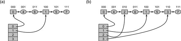
Figure 13.12 This figure explains the recursive nature of the split ordering. Part (a) shows a split-ordered list consisting of two buckets. The array of buckets refer into a single linked list. The split-ordered keys (above each node) are the reverse of the bitwise representation of the items’ keys. The active bucket array entries 0 and 1 have special sentinel nodes within the list (square nodes), while other (ordinary) nodes are round. Items 4 (whose reverse bit order is “001”) and 6 (whose reverse bit order is “011”) are in Bucket 0 since the LSB of the original key, is “0.” Items 5 and 7 (whose reverse bit orders are “101” and “111” respectively) are in Bucket 1, since the LSB of their original key is 1. Part (b) shows how each of the two buckets is split in half once the table capacity grows from 2 buckets to four. The reverse bit values of the two added Buckets 2 and 3 happen to perfectly split the Buckets 0 and 1.
As before, the capacity N of the hash set is always a power of two. The bucket array initially has Capacity 2 and all bucket references are null, except for the bucket at index 0, which refers to an empty list. We use the variable bucketSize to denote this changing capacity of the bucket structure. Each entry in the bucket array is initialized when first accessed, and subsequently refers to a node in the list.
When an item with hash code k is inserted, removed, or searched for, the hash set uses bucket index k (mod N). As with earlier hash set implementations, we decide when to double the table capacity by consulting a policy() method. Here, however, the table is resized incrementally by the methods that modify it, so there is no explicit resize() method. If the table capacity is 2i, then the bucket index is the integer represented by the key’s i least significant bits (LSBs); in other words, each bucket b contains items each of whose hash code k satisfies k = b (mod 2i).
Because the hash function depends on the table capacity, we must be careful when the table capacity changes. An item inserted before the table was resized must be accessible afterwards from both its previous and current buckets. When the capacity grows to 2i+1, the items in bucket b are split between two buckets: those for which k = b (mod 2i+1) remain in bucket b, while those for which k = b + 2i (mod 2i+1) migrate to bucket b + 2i. Here is the key idea behind the algorithm: we ensure that these two groups of items are positioned one after the other in the list, so that splitting bucket b is achieved by simply setting bucket b + 2i after the first group of items and before the second. This organization keeps each item in the second group accessible from bucket b.
As depicted in Fig. 13.12, items in the two groups are distinguished by their ith binary digits (counting backwards, from least-significant to most-significant). Those with digit 0 belong to the first group, and those with 1 to the second. The next hash table doubling will cause each group to split again into two groups differentiated by the (i + 1)st bit, and so on. For example, the items 4 (“100” binary) and 6 (“110”) share the same least significant bit. When the table capacity is 21, they are in the same bucket, but when it grows to 22, they will be in distinct buckets because their second bits differ.
This process induces a total order on items, which we call recursive split-ordering, as can be seen in Fig. 13.12. Given a key’s hash code, its order is defined by its bit-reversed value.
To recapitulate: a split-ordered hash set is an array of buckets, where each bucket is a reference into a lock-free list where nodes are sorted by their bit-reversed hash codes. The number of buckets grows dynamically, and each new bucket is initialized when accessed for the first time.
To avoid an awkward “corner case” that arises when deleting a node referenced by a bucket reference, we add a sentinel node, which is never deleted, to the start of each bucket. Specifically, suppose the table capacity is 2i+1. The first time that bucket b + 2i is accessed, a sentinel node is created with key b + 2i. This node is inserted in the list via bucket b, the parent bucket of b + 2i. Under split-ordering, b + 2i precedes all items of bucket b + 2i, since those items must end with (i + 1) bits forming the value b + 2i. This value also comes after all the items of bucket b that do not belong to b + 2i: they have identical LSBs, but their ith bit is 0. Therefore, the new sentinel node is positioned in the exact list location that separates the items of the new bucket from the remaining items of bucket b. To distinguish sentinel items from ordinary items, we set the most significant bit (MSB) of ordinary items to 1, and leave the sentinel items with 0 at the MSB. Fig. 13.17 illustrates two methods: makeOrdinaryKey(), which generates a split-ordered key for an object, and makeSentinelKey(), which generates a split-ordered key for a bucket index.
Fig. 13.13 illustrates how inserting a new key into the set can cause a bucket to be initialized. The split-order key values are written above the nodes using 8-bit words. For instance, the split-order value of 3 is the bit-reverse of its binary representation, which is 11000000. The square nodes are the sentinel nodes corresponding to buckets with original keys that are 0,1, and 3 modulo 4 with their MSB being 0. The split-order keys of ordinary (round) nodes are exactly the bit-reversed images of the original keys after turning on their MSB. For example, items 9 and 13 are in the “1 mod 4” bucket, which can be recursively split in two by inserting a new node between them. The sequence of figures describes an object with hash code 10 being added when the table capacity is 4 and Buckets 0, 1, and 3 are already initialized.

Figure 13.13 How the add() method places key 10 to the lock-free table. As in earlier figures, the split-order key values, expressed as 8-bit binary words, appear above the nodes. For example, the split-order value of 1 is the bit-wise reversal of its binary representation. In Step (a) Buckets 0, 1, and 3 are initialized, but Bucket 2 is uninitialized. In Step (b) an item with hash value 10 is inserted, causing Bucket 2 to be initialized. A new sentinel is inserted with split-order key 2. In Step (c) Bucket 2 is assigned a new sentinel. Finally, in Step (d), the split-order ordinary key 10 is added to Bucket 2.
The table is grown incrementally, that is, there is no explicit resize operation. Recall that each bucket is a linked list, with nodes ordered based on the split-ordered hash values. As mentioned earlier, the table resizing mechanism is independent of the policy used to decide when to resize. To keep the example concrete, we implement the following policy: we use a shared counter to allow add() calls to track the average bucket load. When the average load crosses a threshold, we double the table capacity.
To avoid technical distractions, we keep the array of buckets in a large, fixed-size array. We start out using only the first array entry, and use progressively more of the array as the set grows. When the add() method accesses an uninitialized bucket that should have been initialized given the current table capacity, it initializes it. While conceptually simple, this design is far from ideal, since the fixed array size limits the ultimate number of buckets. In practice, it would be better to represent the buckets as a multilevel tree structure which would cover the machine’s full memory size, a task we leave as an exercise.
13.3.2 The BucketList Class
Fig. 13.14 shows the fields, constructor, and some utility methods of the BucketList class that implements the lock-free list used by the split-ordered hash set. Although this class is essentially the same as the LockFreeList class, there are two important differences. The first is that items are sorted in recursive-split order, not simply by hash code. The makeOrdinaryKey() and makeSentinelKey() methods (Lines 10 and 14) show how we compute these split-ordered keys. (To ensure that reversed keys are positive, we use only the lower three bytes of the hash code.) Fig. 13.15 shows how the contains() method is modified to use the split-ordered key. (As in the LockFreeList class, the find(x) method returns a record containing the x’s node, if it exists, along with the immediately preceding and subsequent nodes.)
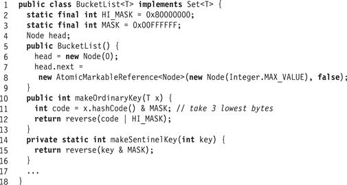
Figure 13.14 BucketList<T> class: fields, constructor, and utilities.

Figure 13.15 BucketList<T> class: the contains() method.
The second difference is that while the LockFreeList class uses only two sentinels, one at each end of the list, the BucketList<T> class places a sentinel at the start of each new bucket whenever the table is resized. It requires the ability to insert sentinels at intermediate positions within the list, and to traverse the list starting from such sentinels. The BucketList<T> class provides a getSentinel(x) method (Fig. 13.16) that takes a bucket index, finds the associated sentinel (inserting it if absent), and returns the tail of the BucketList<T> starting from that sentinel.
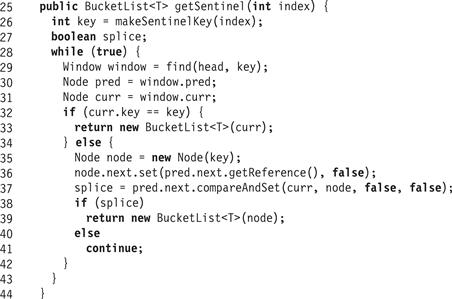
Figure 13.16 BucketList<T> class: getSentinel() method.
13.3.3 The LockFreeHashSet<T> Class
Fig. 13.17 shows the fields and constructor for the LockFreeHashSet<T> class. The set has the following mutable fields: bucket is an array of LockFreeHashSet<T> references into the list of items, bucketSize is an atomic integer that tracks how much of the bucket array is currently in use, and setSize is an atomic integer that tracks how many objects are in the set, used to decide when to resize.
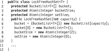
Figure 13.17 LockFreeHashSet<T> class: fields and constructor.
Fig. 13.18 shows the LockFreeHashSet<T> class’s add() method. If x has hash code k, add(x) retrieves bucket k (mod N), where N is the current table size, initializing it if necessary (Line 15). It then calls the BucketList<T>’s add(x) method. If x was not already present (Line 18) it increments setSize, and checks whether to increase bucketSize, the number of active buckets. The contains(x) and remove(x) methods work in much the same way.
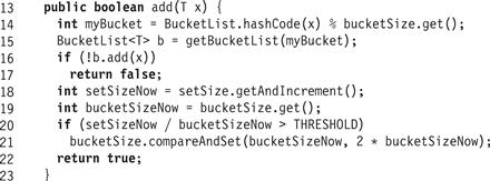
Figure 13.18 LockFreeHashSet<T> class: add() method.
Fig. 13.19 shows the InitializeBucket() method, whose role is to initialize the bucket array entry at a particular index, setting that entry to refer to a new sentinel node. The sentinel node is first created and added to an existing parent bucket, and then the array entry is assigned a reference to the sentinel. If the parent bucket is not initialized (Line 31), InitializeBucket() is applied recursively to the parent. To control the recursion we maintain the invariant that the parent index is less than the new bucket index. It is also prudent to choose the parent index as close as possible to the new bucket index, but still preceding it. We compute this index by unsetting the bucket index’s most significant nonzero bit (Line 39).

Figure 13.19 LockFreeHashSet<T> class: if a bucket is uninitialized, initialize it by adding a new sentinel. Initializing a bucket may require initializing its parent.
The add(), remove(), and contains() methods require a constant expected number of steps to find a key (or determine that the key is absent). To initialize a bucket in a table of bucketSize N, the InitializeBucket() method may need to recursively initialize (i.e., split) as many as O(log N) of its parent buckets to allow the insertion of a new bucket. An example of this recursive initialization is shown in Fig. 13.20. In Part (a) the table has four buckets; only Bucket 0 is initialized. In Part (b) the item with key 7 is inserted. Bucket 3 now requires initialization, further requiring recursive initialization of Bucket 1. In Part (c) Bucket 1 is initialized. Finally, in Part (d), Bucket 3 is initialized. Although the total complexity in such a case is logarithmic, not constant, it can be shown that the expected length of any such recursive sequence of splits is constant, making the overall expected complexity of all the hash set operations constant.

Figure 13.20 Recursive initialization of lock-free hash table buckets. (a) Table has four buckets; only bucket 0 is initialized. (b) We wish to insert the item with key 7. Bucket 3 now requires initialization, which in turn requires recursive initialization of Bucket 1. (c) Bucket 1 is initialized by first adding the 1 sentinel to the list, then setting the bucket to this sentinel. (d) Then Bucket 3 is initialized in a similar fashion, and finally 7 is added to the list. In the worst case, insertion of an item may require recursively initializing a number of buckets logarithmic in the table size, but it can be shown that the expected length of such a recursive sequence is constant.
13.4 An Open-Addressed Hash Set
We now turn our attention to a concurrent open hashing algorithm. Open hashing, in which each table entry holds a single item rather than a set, seems harder to make concurrent than closed hashing. We base our concurrent algorithm on a sequential algorithm known as Cuckoo Hashing.
13.4.1 Cuckoo Hashing
Cuckoo hashing is a (sequential) hashing algorithm in which a newly added item displaces any earlier item occupying the same slot.1 For brevity, a table is a k-entry array of items. For a hash set of size N = 2k we use a two-entry array table[] of tables,2 and two independent hash functions,
![]()
(denoted as hash0() and hash1() in the code) mapping the set of possible keys to entries in the array. To test whether a value x is in the set, contains(x) tests whether either table[0][h0(x)] or table[1][h1(x)] is equal to x. Similarly, remove(x) checks whether x is in either table[0][h0(x)] or table[1][h1(x)], and removes it if found.
The add(x) method (Fig. 13.21) is the most interesting. It successively “kicks out” conflicting items until every key has a slot. To add x, the method swaps x with y, the current occupant of table[0][h0(x)] (Line 6). If the prior value y was null, it is done (Line 7). Otherwise, it swaps the newly nest-less value y for the current occupant of table[1][h1(y)] in the same way (Line 8). As before, if the prior value was null, it is done. Otherwise, the method continues swapping entries (alternating tables) until it finds an empty slot. An example of such a sequence of displacements appears in Fig. 13.22.

Figure 13.21 Sequential Cuckoo Hashing: the add() method.

Figure 13.22 A sequence of displacements started when an item with key 14 finds both locations Table[0][h0(14)] and Table[1][h1(14)] taken by the values 3 and 23, and ends when the item with key 39 is successfully placed in Table[1][h1(39)].
We might not find an empty slot, either because the table is full, or because the sequence of displacements forms a cycle. We therefore need an upper limit on the number of successive displacements we are willing to undertake (Line 5). When this limit is exceeded, we resize the hash table, choose new hash functions (Line 12), and start over (Line 13).
Sequential cuckoo hashing is attractive for its simplicity. It provides constant-time contains() and remove() methods, and it can be shown that over time, the average number of displacements caused by each add() call will be constant. Experimental evidence shows that sequential Cuckoo hashing works well in practice.
13.4.2 Concurrent Cuckoo Hashing
The principal obstacle to making the sequential Cuckoo hashing algorithm concurrent is the add() method’s need to perform a long sequence of swaps. To address this problem, we now define an alternative Cuckoo hashing algorithm, the PhasedCuckooHashSet<T> class. We break up each method call into a sequence of phases, where each phase adds, removes, or displaces a single item x.
Rather than organizing the set as a two-dimensional table of items, we use a two-dimensional table of probe sets, where a probe set is a constant-sized set of items with the same hash code. Each probe set holds at most PROBE_SIZE items, but the algorithm tries to ensure that when the set is quiescent (i.e., no method calls are in progress) each probe set holds no more than THRESHOLD < PROBE_SIZE items. An example of the PhasedCuckooHashSet structure appears in Fig. 13.24, where the PROBE_SIZE is 4 and the THRESHOLD is 2. While method calls are in-flight, a probe set may temporarily hold more than THRESHOLD but never more than PROBE_SIZE items. (In our examples, it is convenient to implement each probe set as a fixed-size List<T>.) Fig. 13.23 shows the PhasedCuckooHashSet<T>’s fields and constructor.

Figure 13.23 PhasedCuckooHashSet<T> class: fields and constructor.
To postpone our discussion of synchronization, the PhasedCuckooHashSet<T> class is defined to be abstract, that is, it does not implement all its methods. The PhasedCuckooHashSet<T> class has the same abstract methods as the BaseHashSet<T> class: The acquire(x) method acquires all the locks necessary to manipulate item x, release(x) releases them, and resize() resizes the set. (As before, we require acquire(x) to be reentrant).
From a bird’s eye view, the PhasedCuckooHashSet<T> works as follows. It adds and removes items by first locking the associated probe sets in both tables. To remove an item, it proceeds as in the sequential algorithm, checking if it is in one of the probe sets and removing it if so. To add an item, it attempts to add it to one of the probe sets. An item’s probe sets serves as temporary overflow buffer for long sequences of consecutive displacements that might occur when adding an item to the table. The THRESHOLD value is essentially the size of the probe sets in a sequential algorithm. If the probe sets already has this many items, the item is added anyway to one of the PROBE_SIZE–THRESHOLD overflow slots. The algorithm then tries to relocate another item from the probe set. There are various policies one can use to choose which item to relocate. Here, we move the oldest items out first, until the probe set is below threshold. As in the sequential cuckoo hashing algorithm, one relocation may trigger another, and so on. Fig. 13.24 shows an example execution of the PhasedCuckooHashSet<T>.

Figure 13.24 The PhasedCuckooHashSet<T> class: add() and relocate() methods. The figure shows the array segments consisting of 8 probe sets of size 4 each, with a threshold of 2. Shown are probe sets 4 and 5 of Table[0][] and 1 and 2 of Table[1][]. In Part (a) an item with key 13 finds Table[0][4] above threshold and Table[1][2] below threshold so it adds the item to the probe set Table[1][2]. The item with key 14 on the other hand finds that both of its probe sets are above threshold, so it adds its item to Table[0][5] and signals that the item should be relocated. In Part (b), the method tries to relocate the item with key 23, the oldest item in Table[0][5]. Since Table[1][1] is below threshold, the item is successfully relocated. If Table[1][1] were above threshold, the algorithm would attempt to relocate item 12 from Table[1][1], and if Table[1][1] were at the probe set’s size limit of 4 items, it would attempt to relocate the item with key 5, the next oldest item, from Table[0][5].
Fig. 13.25 shows the PhasedCuckooHashSet<T> class’s remove(x) method. It calls the abstract acquire(x) method to acquire the necessary locks, then enters a try block whose finally block calls release(x). In the try block, the method simply checks whether x is present in Table[0][h0(x)] or Table[1][h1(x)]. If so, it removes x and returns true, and otherwise returns false. The contains(x) method works in a similar way.
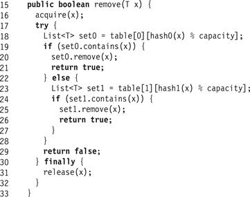
Figure 13.25 PhasedCuckooHashSet<T> class: the remove() method.
Fig. 13.26 illustrates the add(x) method. Like remove(), it calls acquire(x) to acquire the necessary locks, then enters a try block whose finally block calls release(x). It returns false if the item is already present (Line 41). If either of the item’s probe sets is below threshold (Lines 44 and 46), it adds the item and returns. Otherwise, if either of the item’s probe sets is above threshold but not full (Lines 48 and 50), it adds the item and makes a note to rebalance the probe set later. Finally, if both sets are full, it makes a note to resize the entire set (Line 53). It then releases the lock on x (Line 56).
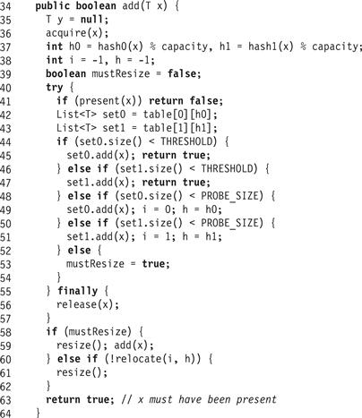
Figure 13.26 PhasedCuckooHashSet<T> class: the add() method.
If the method was unable to add x because both its probe sets were full, it resizes the hash set and tries again (Line 58). If the probe set at row r and column c was above threshold, it calls relocate(r, c) (described later) to rebalance probe set sizes. If the call returns false, indicating that it failed to rebalance the probe sets, then add() resizes the table.
The relocate() method appears in Fig. 13.27. It takes the row and column coordinates of a probe set observed to have more than THRESHOLD items, and tries to reduce its size below threshold by moving items from this probe set to alternative probe sets.
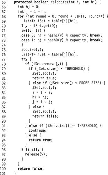
Figure 13.27 PhasedCuckooHashSet<T> class: the relocate() method.
This method makes a fixed number(LIMIT) of attempts before giving up. Each time around the loop, the following invariants hold: iSet is the probe set we are trying to shrink, y is the oldest item in iSet, and jSet is the other probe set where y could be. The loop identifies y (Line 70), locks both probe sets to which y could belong (Line 75), and tries to remove y from the probe set (Line 78). If it succeeds (another thread could have removed y between Lines 70 and 78), then it prepares to add y to jSet. If jSet is below threshold (Line 79), then the method adds y to jSet and returns true (no need to resize). If jSet is above threshold but not full (Line 82), then it tries to shrink jSet by swapping iSet and jSet (Lines 82–86) and resuming the loop. If jSet is full (Line 87), the method puts y back in iSet and returns false (triggering a resize). Otherwise it tries to shrink jSet by swapping iSet and jSet (Lines 82–86). If the method does not succeed in removing y at Line 78, then it rechecks the size of iSet. If it is still over threshold (Line 91), then the method resumes the loop and tries again to remove an item. Otherwise, iSet is below threshold, and the method returns true (no resize needed). Fig. 13.24 shows an example execution of the PhasedCuckooHashSet<T> where the item with key 14 causes a relocation of the oldest item 23 from the probe set table[0][5].
13.4.3 Striped Concurrent Cuckoo Hashing
We first consider a concurrent Cuckoo hash set implementation using lock striping (Chapter 13, Section 13.2.2). The StripedCuckooHashSet class extends PhasedCuckooHashSet, providing a fixed 2-by-L array of reentrant locks. As usual, lock[i][j] protects table[i][k], where k (mod L) = j. Fig. 13.28 shows the StripedCuckooHashSet class’s fields and constructor. The constructor calls the PhasedCuckooHashSet<T> constructor (Line 4) and then initializes the lock array.
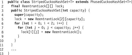
Figure 13.28 StripedCuckooHashSet class: fields and constructor.
The StripedCuckooHashSet class’s acquire(x) method (Fig. 13.29) locks lock[0][h0(x)] and lock[1][h1(x)] in that order, to avoid deadlock. The release(x) method unlocks those locks.
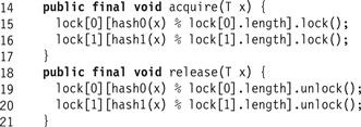
Figure 13.29 StripedCuckooHashSet class: acquire() and release().
The only difference between the resize() methods of StripedCuckooHashSet (Fig. 13.30) and StripedHashSet is that the latter acquires the locks in lock[0]in ascending order (Line 24). Acquiring these locks in this order ensures that no other thread is in the middle of an add(), remove(), or contains() call, and avoids deadlocks with other concurrent resize() calls.
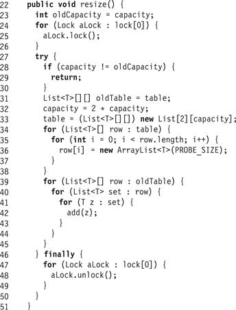
Figure 13.30 StripedCuckooHashSet class: the resize() method.
13.4.4 A Refinable Concurrent Cuckoo Hash Set
We can use the methods of Chapter 13, Section 13.2.3 to resize the lock arrays as well. This section introduces the RefinableCuckooHashSet class (Fig. 13.31). Just as for the RefinableHashSet class, we introduce an owner field of type AtomicMarkableReference<Thread> that combines a Boolean value with a reference to a thread. If the Boolean value is true, the set is resizing, and the reference indicates which thread is in charge of resizing.
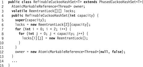
Figure 13.31 RefinableCuckooHashSet<T>: fields and constructor.
Each phase locks the buckets for x by calling acquire(x), shown in Fig. 13.32. It reads the lock array (Line 24), and then spins until no other thread is resizing the set (Lines 21–23). It then acquires the item’s two locks (Lines 27 and 28), and checks if the lock array is unchanged (Line 30). If the lock array has not changed between Lines 24 and 30, then the thread has acquired the locks it needs to proceed. Otherwise, the locks it has acquired are out of date, so it releases them and starts over. The release(x) method releases the locks acquired by acquire(x).
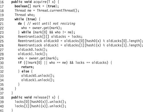
Figure 13.32 RefinableCuckooHashSet<T>: acquire() and release() methods.
The resize() method in (Fig. 13.33) is almost identical to the resize() method for the StripedCuckooHashSet class. One difference is that the locks[] array has two dimensions.
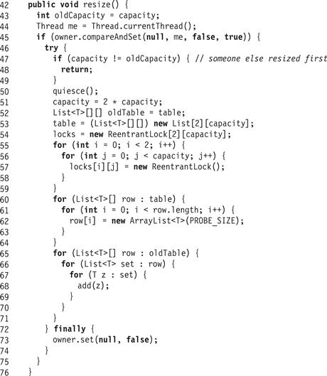
Figure 13.33 RefinableCuckooHashSet<T>: the resize() method.
The quiesce() method, like its counterpart in the RefinableHashSet class, visits each lock and waits until it is unlocked. The only difference is that it visits only the locks in locks[0].
13.5 Chapter Notes
The term disjoint-access-parallelism was coined by Amos Israeli and Lihu Rappoport [76]. Maged Michael [114] has shown that simple algorithms using a reader-writer lock [113] per bucket have reasonable performance without resizing. The lock-free hash set based on split-ordering described in Section 13.3.1 is by Ori Shalev and Nir Shavit [141]. The optimistic and fine-grained hash sets are adapted from a hash set implementation by Doug Lea [99], used in java.util.concurrent.
Other concurrent closed-addressing schemes include Meichun Hsu and Wei-Pang Yang [72], Vijay Kumar [87], Carla Schlatter Ellis [38], and Michael Greenwald [48]. Hui Gao, Jan Friso Groote, and Wim Hesselink [44] propose an almost wait-free extensible open-addressing hashing algorithm and Chris Purcell and Tim Harris [129] propose a concurrent non-blocking hash table with open addressing. Cuckoo hashing is credited to Rasmus Pagh and Flemming Rodler [122], and the concurrent version is by Maurice Herlihy, Nir Shavit, and Moran Tzafrir [68].
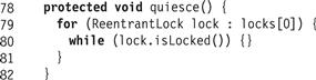
Figure 13.34 RefinableCuckooHashSet<T>: the quiesce() method.
Exercise 158. Modify the StripedHashSet to allow resizing of the range lock array using read/write locks.
Exercise 159. For the LockFreeHashSet, show an example of the problem that arises when deleting an entry pointed to by a bucket reference, if we do not add a sentinel entry, which is never deleted, to the start of each bucket.
Exercise 160. For the LockFreeHashSet, when an uninitialized bucket is accessed in a table of size N, it might be necessary to recursively initialize (i.e., split) as many as O(log N) of its parent buckets to allow the insertion of a new bucket. Show an example of such a scenario. Explain why the expected length of any such recursive sequence of splits is constant.
Exercise 161. For the LockFreeHashSet, design a lock-free data structure to replace the fixed-size bucket array. Your data structure should allow an arbitrary number of buckets.
Exercise 162. Outline correctness arguments for LockFreeHashSet’s add(), remove(), and contains() methods.
Hint: you may assume the LockFreeList algorithm’s methods are correct.
1 Cuckoos are a family of birds (not clocks) found in North America and Europe. Most species are nest parasites: they lay their eggs in other birds’ nests. Cuckoo chicks hatch early, and quickly push the other eggs out of the nest.
2 This division of the table into two arrays will help in presenting the concurrent algorithm. There are sequential Cuckoo hashing algorithms that use, for the same number of hashed items, only a single array of size 2k.