Chapter 14
Heat Transfer and Thermal Insulation
Contents
14.1. Introduction
14.2. Heat Transfer Fundamentals
14.2.1. Heat Conduction
14.2.2. Convection
14.2.2.1. Internal Convection
14.2.2.2. External Convection
14.2.3. Buried Pipeline Heat Transfer
14.2.3.1. Fully Buried Pipeline
14.2.3.2. Partially Buried Pipeline
14.2.4. Soil Thermal Conductivity1
14.3. U-Value
14.3.1. Overall Heat Transfer Coefficient
14.3.2. Achievable U-Values
14.3.3. U-Value for Buried Pipe
14.4. Steady-State Heat Transfer
14.4.1. Temperature Prediction along a Pipeline
14.4.2. Steady-State Insulation Performance
14.5. Transient Heat Transfer
14.5.1. Cooldown
14.5.1.1. Lumped Capacitance Method
14.5.1.2. Finite Difference Method
14.5.2. Transient Insulation Performance
14.6. Thermal Management Strategy and Insulation
14.6.1. External Insulation Coating System
14.6.1.1. Insulation Material
14.6.1.2. Structural Issues
14.6.2. Pipe-in-Pipe System
14.6.3. Bundling
14.6.4. Burial
14.6.5. Direct Heating
14.6.5.1. Closed Return Systems
14.6.5.2. Open Return Systems (Earthed Current)
14.6.5.3. PIP System
14.6.5.4. Hot Fluid Heating (Indirect Heating)
14.1 Introduction
The thermal performance of subsea production systems is controlled by the hydraulic behavior of the fluid in the pipeline; conversely, it also impacts the hydraulic design indirectly through the influence of temperature on fluid properties such as GOR, density, and viscosity. Thermal design, which predicts the temperature profile along the pipeline, is one of the most important parts of pipeline design, because this information is required for pipeline analyses including expansion analysis, upheaval or lateral buckling, corrosion protection, hydrate prediction, and wax deposition analysis. In most cases, the management of the solids (hydrate, wax, asphaltenes, and scales) produced determines the hydraulic and thermal design requirements. To maintain a minimum temperature of fluid to prevent hydrate and wax deposition in the pipeline, insulation layers may be added to the pipeline.
Thermal design includes both steady-state and transient heat transfer analyses. In steady-state operation, the production fluid temperature decreases as it flows along the pipeline due to the heat transfer through the pipe wall to the surrounding environment. The temperature profile in the whole pipeline system should be higher than the requirements for prevention of hydrate and wax formation during normal operation and is determined from steady-state flow and heat transfer calculations. If the steady flow conditions are interrupted due to a shutdown or restarted again during operation, the transient heat transfer analysis for the system is required to make sure the temperature of fluid is out of the solid formation range within the required time. It is necessary to consider both steady-state and transient analyses in order to ensure that the performance of the insulation coatings will be adequate in all operational scenarios.
The thermal management strategy for pipelines can be divided into passive control and active heating. Passive control includes pipelines insulated by external insulation layers, pipe-in-pipe (PIP), bundle and burial; and active heating includes electrical heating and hot fluid heating.
In addition, if the production fluid contains gas, the fluid can experience a temperature drop due to the Joule-Thompson (JT) effect. The JT effect is primarily caused by pressure-head changes, which predominantly occur in the flowline riser and may cause the flowline temperature to fall below ambient temperatures. JT cooling cannot be prevented by insulation. Thus, the JT effect will not be explicitly discussed other than that its effects are implicitly included in some of the numerical results.
The purpose of this chapter is to discuss thermal behavior and thermal management of a pipeline system, which includes,
14.2 Heat Transfer Fundamentals
Figure 14-1 shows the three heat transfer modes occurring in nature: conduction, convection, and radiation. Heat is transferred by any one or a combination of these three modes. When a temperature gradient exists in a stationary medium, which may be gas, liquid, or solid, the conduction will occur across the medium. If a surface and a moving fluid have a temperature difference, the convection will occur between the fluid and surface. All solid surfaces with a temperature will emit energy in the form of electromagnetic waves, which is called radiation. Although these three heat transfer modes occur at all subsea systems, for typical pipelines, heat transfer from radiation is relatively insignificant compared with heat transfer from conduction and convection because the system temperature is below 200°C in generally. Therefore, conduction and convection will be solely considered here.

Figure 14-1 Conduction, Convection, and Radiation Modes [1]
14.2.1 Heat Conduction
For a one-dimensional plane with a temperature distribution T(x), the heat conduction is quantified by the following Fourier equation:
![]() (14-1)
(14-1)
where
q″ : heat flux, Btu/(hr·ft2) or W/m2, heat transfer rate in the x direction per unit area;
k: thermal conductivity of material, Btu/(ft-hr-°F) or W/(m-K);
dT/dx: temperature gradient in the x direction, °F/ft or °C/m.
When the thermal conductivity of a material is constant along the wall thickness, the temperature distribution is linear and the heat flux becomes:
![]() (14-2)
(14-2)
Once the temperature distribution is known, the heat flux at any point in the medium may be calculated from the Fourier equation. By applying an energy balance to a 3D differential control volume and temperature boundary condition, the temperature distribution may be acquired from the heat diffusion equation:
![]() (14-3)
(14-3)
where
![]() : heat generation rate per unit volume of the medium, Btu/(hr·ft3) or W/m3;
: heat generation rate per unit volume of the medium, Btu/(hr·ft3) or W/m3;
ρ: density of the medium, lb/ft3 or kg/m3;
For cylindrical coordinates, the heat diffusion equation may be rewritten as:
![]() (14-4)
(14-4)
where
For most thermal analyses of flowline systems, where the heat transfer along the axial and circumferential directions may be ignored and, therefore, transient heat conduction without a heat source will occur in the radial direction of cylindrical coordinates, the above equation is simplified as follows:
![]() (14-5)
(14-5)
The temperature change rate (∂T/∂t) depends not only on the thermal conductivity of material k, but also on the density, ρ, and specific heat capacity, cp . This equation can be solved numerically. For a steady heat transfer, the right side of equation is equal to zero. The total heat flow per unit length of cylinder is calculated by following equation:
![]() (14-6)
(14-6)
where
14.2.2 Convection
Both internal and external surfaces of a subsea pipeline come in contact with fluids, so convection heat transfer will occur when there is a temperature difference between the pipe surface and the fluid. The convection coefficient is also called a film heat transfer coefficient in the flow assurance field because convection occurs at a film layer of fluid adjacent to the pipe surface.
14.2.2.1 Internal Convection
Internal convection heat transfer occurs between the fluid flowing in a pipe and the pipe internal surface; it depends on the fluid properties, the flow velocity, and the pipe diameter. For the internal convection of pipelines, Dittus and Boelter [2] proposed the following dimensionless correlation for fully turbulent flow of single-phase fluids:
![]() (14-7)
(14-7)
where
n: 0.4 if the fluid is being heated, and 0.3 if the fluid is being cooled;
hi : internal convection coefficient, Btu/(ft2·hr·°F) or W/(m2·K);
Di : pipeline inside diameter, ft or m;
kf : thermal conductivity of the flowing liquid, Btu/(ft·hr·°F) or W/(m·K);
Vf : velocity of the fluid, ft/s or m/s;
ρf : density of the fluid, lb/ft3 or kg/m3;
μf : viscosity of the fluid, lb/(ft·s) or Pa.s;
Cpf : specific heat capacity of the fluid, Btu/(lb·°F) or J/(kg·K).
All fluid properties are assumed to be evaluated at the average fluid temperature. This correlation gives satisfactory results for flows with a Reynolds number greater than 10,000, a Prandtl number of 0.7 to 160, and a pipeline length greater than 10D.
If the flow is laminar (i.e., Rei < 2100), hi may be calculated using Hausen’s equation [3] as follows:
 (14-8)
where Lo is the distance from the pipe inlet to the point of interest. In most pipeline cases, Di /Lo ≈ 0, therefore Equation (14-8) becomes:
![]() (14-9)
(14-9)
For the transition region (2100 < Rei < 104), the heat transfer behavior in this region is always uncertain because of the unstable nature of the flow, especially for multiphase flow in pipeline systems. A correlation proposed by Gnielinski [4] may be used to calculate hi in this region:
![]() (14-10)
(14-10)
where the fiction factor f may be obtained from the Moody diagram, which was discussed in Chapter 13, or for smooth tubes:
![]() (14-11)
(14-11)
This correlation is valid for 0.5 < Pri < 2000 and 3000 < Rei < 5 × 10⁶.
Table 14-1 shows typical ranges for internal convection coefficients for turbulent flow. For most pipelines with multiphase flow, an approximate value of internal convection coefficient based on the table generally is adequate.
Table 14-1. Typical Internal Convection Coefficients for Turbulent Flow [5]
| Fluid | Internal Convection Coefficient, hi | |
| Btu/(ft2·hr·°F) | W/(m2 K) | |
| Water | 300–2000 | 1700–11350 |
| Gases | 3–50 | 17–285 |
| Oils | 10–120 | 55–680 |
Tables 14-2 through 14-5 show thermal conductivities and specific heat capacities for a variety of typical oils and gases. These data can be used for most purposes with sufficient accuracy if these parameters are not known.
Table 14-2. Typical Thermal Conductivities for Crude Oil/Hydrocarbon Liquids [5]

Table 14-3. Typical Thermal Conductivities for Hydrocarbon Gases [5]

Table 14-4. Typical Specific Heat Capacities for Hydrocarbon Liquids [5]
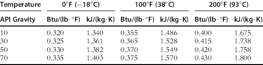
Table 14-5. Typical Specific Heat Capacities for Hydrocarbon Gases [5]

14.2.2.2 External Convection
The correlation of average external convection coefficient suggested by Hilpert [6] is widely used in industry:
![]() (14-12)
(14-12)
where
ho : external convection coefficient, Btu/(ft2·hr·°F) or W/(m2·K);
Do : pipeline outer diameter, ft or m;
ko : thermal conductivity of the surrounding fluid, Btu/(ft·hr·°F) or W/(m·K);
Vo : velocity of the surrounding fluid, ft/s or m/s;
ρo : density of the surrounding fluid, lb/ft3 or kg/m3;
μo : viscosity of the surrounding fluid, lb/(ft·s) or Pa·s;
Cp,o : specific heat capacity of surrounding fluid, Btu/(lb·°F) or J/(kg·K);
C, m : constants, dependent on the Re number range, and listed in Table 14-6.
Table 14-6. Constants of Correlation
| Reo | C | m |
| 4 × 10⁻¹ − 4 × 100 | 0.989 | 0.330 |
| 4 × 100 − 4 × 101 | 0.911 | 0.385 |
| 4 × 101 − 4 ×10³ | 0.683 | 0.466 |
| 4 × 10³ − 4 × 10⁴ | 0.193 | 0.618 |
| 4 × 10⁴ − 4 × 10⁵ | 0.027 | 0.805 |
All of the properties used in the above correlation are evaluated at the temperature of film between the external surface and the surrounding fluid.
When the velocity of surrounding fluid is less than approximately 0.05 m/s in water and 0.5 m/s in air, natural convection will have the dominating influence and the following values may be used:
![]() (14-13)
(14-13)
Note:
• Many of the parameters used in the correlation are themselves dependent on temperature. Because the temperature drop along most pipelines is relatively small, average values for physical properties may be used.
• The analysis of heat transfer through a wall to surrounding fluid does not address the cooling effect due to the Joule-Thompson expansion of a gas. For a long gas pipeline or pipeline with two-phase flow, an estimation of this cooling effect should be made.
14.2.3 Buried Pipeline Heat Transfer
Pipeline burial in subsea engineering occurs for these reasons:
• Placement of rock, grit, or seabed material on the pipe for stability and protection requirements;
• Gradual infill due to sediment of a trenched pipeline;
• General embedment of the pipeline into the seabed because of the seabed mobility or the pipeline movement.
Although seabed soil can be a good insulator, porous burial media, such as rock dump, may provide little insulation because water can flow through the spaces between the rocks and transfer heat to the surroundings by convection.
14.2.3.1 Fully Buried Pipeline
For a fully buried pipeline, the heat transfer is not symmetrical. To simulate a buried pipeline, a pseudo-thickness of the soil is used to account for the asymmetries of the system in pipeline heat transfer simulation software such as OLGA and PIPESIM.
By using a conduction shape factor for a horizontal cylinder buried in a semi-infinite medium, as shown in Figure 14-2, the heat transfer coefficient for a buried pipeline can be expressed as:
![]() (14-14)
(14-14)
where
hsoil: heat transfer coefficient of soil, Btu/ (ft2·hr·°F) or W/ (m2·K);
ksoil: thermal conductivity of soil, Btu/(ft·hr·°F) or W/(m·K);
D: outside diameter of buried pipe, ft or m;
Z: distance between top of soil and center of pipe, ft or m.

Figure 14-2 Cross Section of a Buried Pipeline
For the case of Z > D/2, cosh–1(2Z/D) can be simplified as ln[(2Z/D) + ((2Z/D) 2 –1)0.5]; therefore:
![]() (14-15)
(14-15)
14.2.3.2 Partially Buried Pipeline
The increase in the insulation effect for a partially buried pipeline is not large compared with a fully buried pipeline. Heat flows circumferentially through the steel to the section of exposure. Even exposure of just the crown of the pipeline results in efficient heat transfer to the surroundings due to the high thermal conductivity of the steel pipe. A trenched pipeline (partially buried pipeline) experiences less heat loss than an exposed pipeline but more than a buried pipeline. Engineering judgment must be used for the analysis of trenched pipelines. Seabed currents may be modified to account for the reduced heat transfer, or the heat transfer may be calculated using a weighted average of the fully buried pipe and exposed pipe as follows:
![]() (14-16)
(14-16)
where f is the fraction of outside surface of pipe exposed to the surrounding fluid, and ho is the external heat transfer coefficient, Btu/(ft2·hr·°F) or W/(m2·K).
For an exposed pipeline the theoretical approach assumes that water flows over the top and bottom of the pipeline. For concrete-coated pipelines, where the external film coefficient has little effect on the overall heat transfer coefficient, the effect of resting on the seabed is negligible. However, for pipelines without concrete coatings these effects must be considered.
A pipeline resting on the seabed is normally assumed to be fully exposed. A lower heat loss can give rise to upheaval buckling, increased corrosion, and overheating of the coating. It is necessary to take into account the changes in burial levels over field life and, hence, the changes in insulation values.
14.2.4 Soil Thermal Conductivity
Soil thermal conductivity has been found to be a function of dry density, saturation, moisture content, mineralogy, temperature, particle size/shape/arrangement, and the volumetric proportions of solid, liquid, and air phases. A number of empirical relationships (e.g., Kersten [7]) have been developed to estimate thermal conductivity based on these parameters. For a typical unfrozen silt-clay soil, the Kersten correlation is expressed as follows:
![]() (14-17)
(14-17)
where
κsoil : soil thermal conductivity, Btu·in./(ft2·hr·°F);
The above correlation was based on the data for five soils and is valid for moisture contents of 7 percent or higher.
Table 14-7 lists the thermal conductivities of typical soils surrounding pipelines. Although the thermal conductivity of onshore soils has been extensively investigated, until recently there has been little published thermal conductivity data for deepwater soil (e.g., Power et al. [8], Von Herzen and Maxwell [9]). Many deepwater offshore sediments are formed with predominantly silt- and clay-sized particles, because sand-sized particles are rarely transported this far from shore. Hence, convective heat loss is limited in these soils, and the majority of heat transfer is due to conduction [10]. Recent measurements of thermal conductivity for deepwater soils from the Gulf of Mexico [11] have shown values in the range of 0.7 to 1.3 W/(m·K), which is lower than that previously published for general soils and is approaching that of still seawater, 0.65 W/(m·K). This is a reflection of the very high moisture content of many offshore soils, where liquidity indices well in excess of unity can exist and which are rarely found onshore. Although site-specific data are needed for the detailed design most deepwater clay is fairly consistent. Figure 14-3 shows sample thermal conductivity test results for subsea soils worldwide. The sample results prove that most deepwater soils have similar characteristics.
Table 14-7. Thermal Conductivities of Typical Soil Surrounding Pipeline [5]
| Material | Thermal Conductivity, ksoil | |
| Btu/(ft·hr·°F) | W/(m·K) | |
| Peat (dry) | 0.10 | 0.17 |
| Peat (wet) | 0.31 | 0.54 |
| Peat (icy) | 1.09 | 1.89 |
| Sand soil (dry) | 0.25–0.40 | 0.43–0.69 |
| Sandy soil (moist) | 0.50–0.60 | 0.87–1.04 |
| Sandy soil (soaked) | 1.10–1.40 | 1.90–2.42 |
| Clay soil (dry) | 0.20–0.30 | 0.35–0.52 |
| Clay soil (moist) | 0.40–0.50 | 0.69–0.87 |
| Clay soil (wet) | 0.60–0.90 | 1.04–1.56 |
| Clay soil (frozen) | 1.45 | 2.51 |
| Gravel | 0.55–0.72 | 0.9–1.25 |
| Gravel (sandy) | 1.45 | 2.51 |
| Limestone | 0.75 | 1.30 |
| Sandstone | 0.94 –1.20 | 1.63–2.08 |

Figure 14-3 Sample Soil Thermal Conductivity Test Results for Offshore Soils Worldwide [12]
14.3 U-Value
14.3.1 Overall Heat Transfer Coefficient
Figure 14-4 shows the temperature distribution of a cross section for a composite subsea pipeline with two insulation layers. Radiation between the internal fluid and the pipe wall and the pipeline outer surface and the environment is ignored because of the relatively low temperature of subsea systems.

Figure 14-4 Cross Section of Insulated Pipe and Temperature Distribution
Convection and conduction occur in an insulated pipeline as follows:
• Convection from the internal fluid to the pipeline wall;
• Conduction through the pipe wall and exterior coatings, and/or to the surrounding soil for buried pipelines;
• Convection from flowline outer surface to the external fluid.
For internal convection at the pipeline inner surface, the heat transfer rate across the surface boundary is given by the Newton equation:
![]() (14-18)
(14-18)
where
Qi : convection heat transfer rate at internal surface, Btu/hr or W;
hi : internal convection coefficient, Btu/(ft2·hr·°F) or W/(m2·K);
ri : internal radius of flowline, ft or m;
Ai : internal area normal to the heat transfer direction, ft2 or m2;
For external convection at the pipeline outer surface, the heat transfer rate across the surface boundary to the environment is:
![]() (14-19)
(14-19)
where
Qo : convection heat transfer rate at outer surface, Btu/hr or W;
ho : outer convection coefficient, Btu/(ft2·hr·°F) or W/(m2·K);
ro : outer radius of flowline, ft or m;
Ao : outer area normal to the heat transfer direction, ft2 or m2;
Conduction in the radial direction of a cylinder can be described by Fourier’s equation in radial coordinates:
![]() (14-20)
(14-20)
where
Qr : conduction heat transfer rate in radial direction, Btu/hr or W;
r: radius of cylinder, ft or m;
k: thermal conductivity of cylinder, Btu/(ft·hr·°F) or W/(m·K);
Integration of Equation (14-20) gives:
![]() (14-21)
(14-21)
The temperature distribution in the radial direction can be calculated for steady-state heat transfer between the internal fluid and pipe surroundings where heat transfer rates of internal convection, external convection, and conduction are the same. The following heat transfer rate equation is obtained:
![]() (14-22)
(14-22)
The heat transfer rate through a pipe section with length of L, due to a steady-state heat transfer between the internal fluid and the pipe surroundings, is also expressed as follows:
![]() (14-23)
(14-23)
where
U: overall heat transfer coefficient (OHTC), based on the surface area A,
Btu/ (ft2·hr·°F) or W/ (m2·K);
A: area of heat transfer surface, Ai or Ao , ft2 or m2;
To : ambient temperature of the pipe surroundings, °F or °C;
Ti : average temperature of the flowing fluid in the pipe section, °F or °C.
Therefore, the OHTC based on the flowline internal surface area Ai is:
![]() (14-24)
(14-24)
and the OHTC based on the flowline outer surface area Ao is:
![]() (14-25)
(14-25)
The OHTC of the pipeline is also called the U-value of the pipeline in subsea engineering. It is a function of many factors, including the fluid properties and fluid flow rates, the convection nature of the surroundings, and the thickness and properties of the pipe coatings and insulation. Insulation manufacturers typically use a U-value based on the outside diameter of a pipeline, whereas pipeline designers use a U-value based on the inside diameter. The relationship between these two U-values is:
![]() (14-26)
(14-26)
The U-value for a multilayer insulation coating system is easily obtained from an electrical-resistance analogy between heat transfer and direct current. The steady-state heat transfer rate is determined by:
![]() (14-27)
(14-27)
where UA is correspondent with the reverse of the cross section’s thermal resistivity that comprises three primary resistances: internal film, external film, and radial material conductance. The relationship is written as follows:
![]() (14-28)
(14-28)
The terms on the right hand side of the above equation represent the heat transfer resistance due to internal convection, conduction through steel well of pipe, conduction through insulation layers and convection at the external surface. They can be expressed as follows.
![]() (14-29)
(14-29)
![]() (14-30)
(14-30)
![]() (14-31)
(14-31)
![]() (14-32)
(14-32)
whererno and rni represent the outer radius and inner radius of the coating layer n, respectively. The term kn represents the thermal conductivity of coating layer n, Btu/(ft-hr-°F) or W/(m-K). The use of U-values is appropriate for steady-state simulations. However, U-values cannot be used to evaluate transient thermal simulations; the thermal diffusion coefficient and other material properties of the wall and insulation must be included.
14.3.2 Achievable U-Values
The following U-values are lowest possible values to be used for initial design purposes:
• Conventional insulation: 0.5 Btu/ft2·hr·°F (2.8 W/m2·K);
• Polyurethane pipe-in-pipe: 0.2 Btu/ft2·hr·°F (1.1 W/m2·K);
• Ceramic insulated pipe-in-pipe: 0.09 Btu/ft2·hr·°F (0.5 W/m2·K);
Insulation materials exposed to ambient pressure must be qualified for the water depth where they are to be used.
14.3.3 U-Value for Buried Pipe
For insulated pipelines, a thermal insulation coating and/or burial provide an order of magnitude more thermal resistance than both internal and external film coefficients. Therefore, the effects of internal and external film coefficients on the U-value of pipelines can be ignored. The U-value of pipelines can be described as:
![]() (14-33)
(14-33)
where the first term in the denominator represents the thermal resistance of the radial layers of steel and insulation coatings, and the second term in the denominator represents the thermal resistivity due to the soil and is valid for H > Do /2. If the internal and external film coefficients are to be included, the external film coefficient is usually only included for nonburied pipelines. For buried bare pipelines, where the soil provides essentially the entire pipeline’s thermal insulation, there is a near linear relationship between the U-value and ksoil. For buried and insulated pipelines, the effect of ksoil on the U-value is less than that for buried bare pipelines.
Figure 14-5 presents the relationship between U-value and burial depth for both a bare pipe and a 2-in. polypropylene foam (PPF)-coated pipe. The U-value decreases very slowly with the burial depth, when the ratio of burial depth to outer diameter is greater than 4.0. Therefore, it is not necessary to bury the pipeline to a great depth to get a significant thermal benefit. However, practical minimum and maximum burial depth limitations are applied to modern pipeline burial techniques. In addition, issues such as potential seafloor scouring and pipeline upheaval buckling need to be considered in designing the appropriate pipeline burial depth.

Figure 14-5 U-Value versus Burial Depth for Bare Pipe and 2–In. PPF-Coated Pipe [13]
14.4 Steady-State Heat Transfer
Steady-state thermal design is aimed at ensuring a given maximum temperature drop over a length of insulated pipe. In the steady-state condition, the flow rate of a flowing fluid and heat loss through the pipe wall from the flowing fluid to the surroundings are assumed to be constant at any time.
14.4.1 Temperature Prediction along a Pipeline
The accurate predictions of temperature distribution along a pipeline can be calculated by coupling velocity, pressure, and enthalpy given by mass, momentum, and energy conservation. The complexity of these coupled equations prevents an analytical solution, but they can be solved by a numerical procedure [14].
Figure 14-6 shows a control volume for internal flow for a steady-state heat transfer analysis. In a fully developed thermal boundary layer region of a flowline, the velocity and temperature radial profiles of a single-phase fluid are assumed to be approximately constant along the pipeline. A mean temperature can be obtained by integrating the temperatures over the cross section, and the mean temperature profile of fluid along the pipeline is obtained by the energy conservation between the heat transfer rate through the pipe wall and the fluid thermal energy change as the fluid is cooled by conduction of heat through the pipe to the sea environment, which is expressed as follows:
![]() (14-34)
(14-34)
where
dA : surface area of pipeline, dA = Pdx = π Ddx, ft2 or m2;
![]() : mass flow rate of internal fluid, lb/s or kg/s;
: mass flow rate of internal fluid, lb/s or kg/s;
cp : specific heat capacity of internal fluid, Btu/(lb·°F) or J/(kg·K);

Figure 14-6 Control Volume for Internal Flow in a Pipe [1]
Separating the variables and integrating from the pipeline inlet to the point with a pipe length of x from the inlet, we obtain:
![]() (14-35)
(14-35)
where
Tin : inlet temperature of fluid, °F or °C;
T(x) : temperature of fluid at distance x from inlet, °F or °C.
From integration of Equation (14-35), the following temperature profile equation is obtained:
![]() (14-36)
(14-36)
Here, the thermal decay constant, β, is defined as:
![]() (14-37)
(14-37)
where L is the total pipeline length, ft or m.
However, if two temperatures and their corresponding distance along the route are known, fluid properties in the thermal decay constant are not required. The inlet temperature and another known temperature are used to predict the decay constant and then develop the temperature profile for the whole line based on the exponential temperature profile that is given by the following equation:
![]() (14-38)
(14-38)
If the temperature drop due to Joule-Thompson cooling is taken into account and a single-phase viscous flow is assumed, the temperature along the flowline may be expressed as:
![]() (14-39)
(14-39)
where
14.4.2 Steady-State Insulation Performance
The following insulation methods are used in the field for subsea pipelines:
The most popular methods used in subsea pipeines are external coatings, PIP, and pipeline burial.
Table 14-8 presents the U-values for various pipe size and insulation system combinations. Bare pipe has little resistance to heat loss, but buried bare pipe is equivalent to adding approximately 60 mm of external coating of PPF. Combining burial and coating (B&C) achieves U-values near those of PIP. If lower soil thermal conductivity and/or thicker external coating are used, the B&C system can achieve the same level U-value as typical PIPs. Considering realistic fabrication and installation limitations, PIPs are chosen and designed in most cases to have a lower U-value than B&C. However, the fully installed costs of equivalent PIP systems are estimated to be more than double those of B&C systems.
Table 14-8. U-Values for Different Subsea Insulation Systems [13]

14.5 Transient Heat Transfer
Transient heat transfer occurs in subsea pipelines during shutdown (cooldown) and start-up scenarios. In shutdown scenarios, the energy, kept in the system at the moment the fluid flow stops, goes to the surrounding environment through the pipe wall. This is no longer a steady-state system and the rate at which the temperature drops with time becomes important to hydrate control of the pipeline.
Pipeline systems are required to be designed for hydrate control in the cooldown time, which is defined as the period before the pipeline temperature reaches the hydrate temperature at the pipeline operating pressure. This period provides the operators with a decision time in which to commence hydrate inhibition or pipeline depressurization. In the case of an emergency shutdown or cooldown, it also allows for sufficient time to carry out whatever remedial action is required before the temperature reaches the hydrate formation temperature. Therefore, it is of interest to be able to predict how long the fluid will take to cool down to any hydrate formation temperature with a reasonable accuracy. When a pipeline is shut down for an extended period of time, generally it is flushed (blown down) or vented to remove the hydrocarbon fluid, because the temperature of the system will eventually come to equilibrium with the surroundings.
The cooldown process is a complex transient heat transfer problem, especially for multiphase fluid systems. The temperature profiles over time may be obtained by considering the heat energy resident in the fluid and the walls of the system, ![]() , the temperature gradient over the walls of the system, and the thermal resistances hindering the heat flow to the surroundings. The software OLGA is widely used for numerical simulation of this process. However, OLGA software generally takes several hours to do these simulations. In many preliminary design cases, an analytic transient heat transfer analysis of the pipeline, for example, the lumped capacitance method, is fast and provides reasonable accuracy.
, the temperature gradient over the walls of the system, and the thermal resistances hindering the heat flow to the surroundings. The software OLGA is widely used for numerical simulation of this process. However, OLGA software generally takes several hours to do these simulations. In many preliminary design cases, an analytic transient heat transfer analysis of the pipeline, for example, the lumped capacitance method, is fast and provides reasonable accuracy.
14.5.1 Cooldown
The strategies for solving the transient heat transfer problems of subsea pipeline systems include analytical methods (e.g., lumped capacitance method), the finite difference method (FDM), and the finite element method (FEM). The method chosen depends on the complexity of the problem. Analytical methods are used in many simple cooldown or transient heat conduction problems. The FDM is relatively fast and gives reasonable accuracy. The FEM is more versatile and better for complex geometries; however, it is also more demanding to implement. A pipe has a very simple geometry; hence, obtaining a solution to the cooldown rate question does not require the versatility of the FEM. For such systems, the FDM is convenient and has adequate accuracy. Valves, bulkheads, Christmas trees, etc., have more complex geometries and require the greater versatility and 3D capability of FEM models.
14.5.1.1 Lumped Capacitance Method
A commonly used mathematical model for the prediction of system cooldown time is the lumped capacitance model, which can be expressed as follows:
![]() (14-40)
(14-40)
where
T: temperature of the body at time t, °F or °C;
To : ambient temperature, °F or °C;
Ti : initial temperature, °F or °C;
D: inner diameter or outer diameter of the flowline, ft or m;
L: length of the flowline, ft or m;
U: U-value of the flowline based on diameter D, Btu/ft2·hr·°F or W/m2·K;
m: mass of internal fluid or coating layers, lb or kg;
cp : specific heat capacity of fluid or coating layers, Btu/(lb·°F) or J/(kg·K).
This model assumes, however, a uniform temperature distribution throughout the object at any moment during the cooldown process and that there is no temperature gradient inside of the object. These assumptions mean that the surface convection resistance is much larger than the internal conduction resistance, or the temperature gradient in the system is negligible. This model is only valid for Biot (Bi) numbers less than 0.1. The Bi number is defined as the ratio of internal heat transfer resistance to external heat transfer resistance and may be written as:
![]() (14-41)
(14-41)
where
Because most risers and pipelines are subject to large temperature gradients across their walls and are also subject to wave and current loading, this leads to a Bi number outside the applicable range of the “lumped capacitance” model. A mathematical model is therefore required that takes into account the effects of external convection on the transient thermal response of the system during a shutdown event.
14.5.1.2 Finite Difference Method
Considering the pipe segment shown earlier in Figure 14-4, which has length L, it is assumed that the average fluid temperature in the segment is Tf,o at a steady-state flowing condition. The temperature of the surroundings is assumed to be Ta , and constant.
Under the steady-state condition, the total mass of the fluid in the pipe segment is given by:
![]() (14-42)
(14-42)
where
Wf : fluid mass in the pipe segment, lb or kg;
Di : pipe inside diameter, in or m;
L: length of the pipe segment, in or m;
ρf: average density of the fluid in the pipe segment when the temperature is Tf,o , lb/in3 or kg/m3.
Note that Wf is assumed to be constant at all times after shutdown. At any given time, the heat content of the fluid in the pipe segment is given by:
![]() (14-43)
(14-43)
where
Cp,f : specific heat of the fluid, Btu/(lb·°F) or kJ/(kg °C);
Tref : a constant reference temperature, °F or °C;
Tf : average temperature of fluid in the pipe segment, °F or °C.
The heat content of the pipe wall and insulation layers can be expressed in the same way:
![]()
![]() (14-44)
(14-44)
An energy balance is applied to the control volume and is used to find the temperature at its center. It is written in the two forms shown below, the first without Fourier’s law of heat conduction. Notice from the equation that during cooldown the quantity of heat leaving is larger than the quantity of heat entering.
In the analysis of heat transfer in a pipeline system, heat transfer along the axial and circumferential directions of the pipeline can be ignored, therefore, the transient heat transfer without heat source occurs only in the radial direction. The first law of thermodynamics states that the change of energy inside a control volume is equal to the heat going out minus the heat entering. Therefore, the heat transfer balance for all parts (including the contained fluid, steel pipe, insulation materials, and coating layers) of the pipeline can be explicitly expressed as in following equation:
![]() (14-45)
(14-45)
where
Qi,0 : heat content of the part i at one time instant, Btu or J;
Qi,1 : heat content of the part i after one time step, Btu or J;
q i+1/2: heat transfer rate from part i to part i+1 at the “0” time instant, Btu/hr or W;
q i−1/2: heat transfer rate from part i – 1 to part i at the “0” time instant, Btu/hr or W;
If the heat transfer rate through all parts of a pipeline system in the radial direction is expressed with the thermal resistant concept, then:
![]() (14-46)
(14-46)
![]() (14-47)
(14-47)
Therefore, the average temperatures for a pipeline with two insulation layers after one time step are rewritten as:
![]() (14-48)
(14-48)
![]() (14-49)
(14-49)
![]() (14-50)
(14-50)
![]() (14-51)
(14-51)
The solution procedure of a finite difference method is based on a classical implicit procedure that uses matrix inversion. The main principle used to arrive at a solution is to find the temperature at each node using the energy equation above. Once an entire row of temperatures has been found at the same time step by matrix inversion, the procedure jumps to the next time step. Finally, the temperature at all time steps is found and the cooldown profile is established. The detailed calculation method and definitions are provided in the Mathcad worksheet in the Appendix at the end of this chapter.
To get an accurate transient temperature profile, the fluid and each insulation layer may be divided into several layers and the above calculation method applied. By setting the exponential temperature profile along the pipeline, obtained from the steady-state heat transfer analysis, as the initial temperature distribution for a cooldown transient analysis, the temperature profiles along the pipeline at different times can be calculated. This methodology is easily programmed as an Excel macro or with C++ or another computer language, but the more layers the insulation is divided into, the shorter the time step required to obtain a convergent result, because an explicit difference is used in the time domain. The maximum time step may be calculated using following equation:
![]() (14-52)
(14-52)
If the layer is very thin, Ri will be very small, which controls the maximum time step. In this case, the thermal energy saved in this layer is very small and may be ignored. The model implemented here conservatively assumes that the content of the pipe has thermal mass only, but no thermal resistance. The thermal energy of the contents is immediately available to the steel. The effect of variations of Cp and k for all parts in the system is of great importance to the accuracy of the cooldown simulation. For this reason, these effects are either entered in terms of fitted expressions or fixed measured quantities. Figure 14-7 shows the variation of measured specific heat capacity for a polypropylene solid with material temperature.

Figure 14-7 Specific Heat Capacity Measurements for Generic Polypropylene Solid
Guo et al. [15] developed a simple analysis model for predicting heat loss and temperature profiles in insulated thermal injection lines and wellbores. The concept of this model is similar to that of the finite difference method described earlier. The model can accurately predict steady-state and transient heat transfer of the well tube and pipeline.
14.5.2 Transient Insulation Performance
Although steady-state performance is generally the primary metric for thermal insulation design, transient cooldown is also important, especially when hydrate formation is possible. Figure 14-8 presents the transient cooldown behavior at the end of a 27-km flowline.

Figure 14-8 Transient Cooldown Behavior between Burial Pipe and PIP [13]
For the case presented in Figure 14-8, the PIP flowline had a slightly lower U-value than that of the B&C flowline. Therefore, the steady-state temperature at the base of the riser is slightly higher for the PIP than the B&C flowline. These steady-state temperatures are the initial temperatures at the start of a transient shutdown. However, the temperature of a B&C system quickly surpasses that of the PIP system and provides much longer cooldown times in the region of typical hydrate formation. For the case considered, the B&C flowline had approximately three times the cooldown time of the PIP before hydrate formation. The extra time available before hydrate formation has significant financial implications for offshore operations, such as reduced chemical injection, reduced line flushing, and reduced topside equipment.
The temperature of the PIP at initial cooldown condition is higher than that of the B&C flowline, but the cooldown curves cross as shown in Figure 14-8. In addition to the U-value, the fluid temperature variation with time is dependent on the fluid’s specific heat, Cp , its mass flow rate, and the ambient temperature.
14.6 Thermal Management Strategy and Insulation
As oil/gas production fields move into deeper water, there is a growing need for thermal management to prevent the buildup of hydrate and wax formations in subsea systems. The thermal management strategy is chosen depending on the required U-value, cooldown time, temperature range, and water depth. Table 14-9 summarizes the advantages, disadvantages, and U-value range of the thermal management strategies used in subsea systems.
Table 14-9. Summary of Thermal Management Strategies for Subsea Systems [16]


Figure 14-9 summarizes subsea pipeline systems with respect to length and U-value, which concludes:
• U-values of single pipe insulation systems are higher than 2.5 W/m2·K, and mostly installed using reeled pipe installation methods;
• About 6 different operating PIP systems with lengths of less than 30 km;
• Reeled PIP systems have dominated the 5- to 20-km market with U-values of 1 to 2 W/m2·K;
• PIP system in development with length of 66 km offers a U-value of 0.5-1.0 W/m2·K;
• About 3 bundles used on tie-backs of over 10 km, with Britannia also incorporating a direct heating system.

Figure 14-9 Field Development versus Pipeline Length and U-Value [18]
14.6.1 External Insulation Coating System
Figure 14-10 shows a typical multilayer coating system that combines the foams with good thermal insulating properties and polypropylene (PP) shield with creep resistance. These coatings vary in thickness from 25 up to 100 mm or more. Typically thicknesses over about 65 mm are applied in multiple layers.
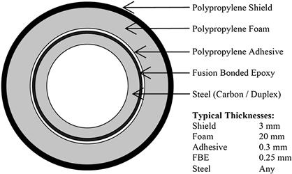
Figure 14-10 Typical Multilayer Insulation System [18]
Coating systems are usually limited by a combination of operating conditions including temperature, water depth, and water absorption. Combinations of temperature and hydrostatic pressure can cause creep and water absorption, with resultant compression of the coating and a continuing reduction in insulating properties throughout the design life. These issues need to be accounted for during the design stage.
Pipelines can be classified according to the pipeline temperature. Table 14-10 shows various temperature ranges with their corresponding insulation materials. Finding suitable thermal insulation for high-temperature subsea pipelines is challenging compared to finding it for lower temperature applications.
Table 14-10. Possible Coating Systems for Thermal Insulation of Flowlines [19]
| Flowline | Temperature Range (°C) | Insulation System |
| Low temperature | –10–70 | Polyurethane (PU), polypropylene (PP), filled rubbers, syntactic foams based on epoxy and polyurethanes |
| Medium temperature | 70–120 | PP, rubber, syntactic epoxy foams |
| High temperature | 120–200 | PP systems, phenolic foams, PIP with polyurethane foam or inorganic insulating materials. |
14.6.1.1 Insulation Material
Table 14-11 summarizes the insulation types, limitations, and characteristics of the most commonly applied and new systems being offered by suppliers. The systems have progressed significantly in the past 10 years on issues such as thickness limits, water depth limitations, impact resistance, operating temperature limits, creep with resultant loss of properties, suitability for reel-lay installation with high strain loading, life expectancy, and resultant U-values and submerged weight.
Table 14-11. External Insulation Systems [18]


Note 1: For multilayer coatings the properties quoted are for the insulation layer.Note 2: Value measured at mean product temperature of 50°C.Note 3: Values are approximate only. All values used in design must be provided by the manufacturer.
Brief descriptions of external insulation systems for subsea systems are as follows:
• Polypropylene (PP): polyolefin system with relatively low thermal efficiency. Applied in three to four layers, can be used in conjunction with direct heating systems. Specific heat capacity is 2000 J/(kg·K).
• Polypropylene-foam (PPF), Solid polypropylene (SPP): Controlled formation of gas bubbles is used to reduce the thermal conductivity; however, as ocean depth and temperature increase, rates of compression and material creep increase. Generally not used on its own.
• Polypropylene-reinforced foam combination (RPPF): A combination of the above two systems incorporating an FBE layer, PPF, and an outer layer of PP to minimize creep and water absorption.
• Polyurethane (PU): A polyolefin system with relatively low thermal efficiency; has a relatively high water absorption as the temperature rises over 50°C. Commonly applied with modified stiffness properties to field joints.
• Polyurethane-syntactic (SPU): One of the most commonly applied systems over recent years; offers good insulation properties at water depths less than 100 m. Specific heat capacity is 1500 J/(kg·K).
• Polyurethane-glass syntactic (GSPU): Similar to SPU but incorporates glass providing greater creep resistance. Specific heat capacity is 1700 J/(kg·K).
• Phenolic syntactic (PhS), epoxy syntactic (SEP), and epoxy syntactic with mini-spheres (MSEP): Based on epoxy and phenolic materials, which offer improved performance at higher temperatures and pressures. These materials are generally applied by trowel or are precast or poured into molds. For example, SEP was used on the 6-mile Shell King development in GoM by pouring the material under a vacuum into polyethylene sleeves. Specific heat capacity is 1240 (J/kg K) [20].
PP and PU are the main components of insulation coating systems. The syntactic insulations that incorporate spheres are used to improve insulation strength for hydrostatic pressure.
14.6.1.2 Structural Issues
Installation and Operation Loads
Coating systems that will be installed by the reeling method need to be carefully selected and tested, because some systems have experienced cracking particularly at field joints where there is a natural discontinuity in the coating. This can lead to strain localization and pipe buckling. Laying and operation of subsea pipelines require a load transfer through the coating to the steel pipe and from the steel pipe to the coating. The coating should have a sufficient shear load capacity to hold the steel pipe during the laying process. Thermal fluctuations in the operation process lead to expansion and contraction of the pipe. The thermal insulation coating is required to allow for such changes without being detached or cracked. These requirements have resulted in most thermal insulation systems being based on bonded geometries, comprised of several layers or cast-in shells.
Hydrostatic Loads
Deepwater pipelines are subject to significant hydrostatic loading due to the extreme water depths. The thermal insulation system must be designed to withstand these large hydrostatic loads. The layer of foamed thermal insulation is the weakest member of the insulation system and therefore the structural response of the insulation system will depend largely on this layer. Elastic deformation of the system leads to a reduction in volume of the insulation system and an increase in density and thermal conductivity of the foam layer, which leads to an increase in the U-value of the system. To reduce the elastic deformation of the system, stiffer materials are required. The stiffness of the foams increases with increasing density. Therefore, to reduce elastic deformation of the system, higher density foams are required.
Creep
Thermal insulation operating in deep water depths for long periods (e.g., 20 to 30 years) is subject to significant creep loading. Creep of thermal insulation can lead to some damaging effects, such as structural instability leading to collapse and also loss of thermal performance. Creep of polymer foams leads to a reduction in volume or densification of the foam. The increased density of the material leads to an increased thermal conductivity and, therefore, the effectiveness of the insulation system is reduced. To design effective thermal insulation systems for deepwater applications, the creep response of the insulating foam must be known.
The factors affecting the creep response of polymer foams include temperature, density, and stress level. The combination of high temperatures and high stresses can accelerate the creep process. High-density foams are desirable for systems subject to large hydrostatic loads for long time periods.
The design of thermal insulation systems for deepwater applications is complex and involves a number of thermal and structural issues. These thermal and structural issues can sometimes conflict. To design effective thermal insulation systems, the thermal and structural issues involved must be carefully considered to achieve a balance. For long-distance tie-backs, the need for a substantial thickness of insulation will obviously have an impact on the installation method due to the increase in pipe outside diameter and the pipe field-jointing process. Because most insulation systems are buoyant, the submerged weight of the pipe will decrease. It may be necessary to increase pipe wall thickness to achieve a submerged weight suitable for installation and on-bottom stability.
14.6.2 Pipe-in-Pipe System
A method of achieving U-values of 1 W/m2·K or less requires PIP insulation systems, in which the inner pipe carrying the fluid is encased within a larger outer pipe. The outer pipe seals the annulus between the two pipes and the annulus can be filled with a wide range of insulating materials that do not have to withstand hydrostatic pressure.
The key features for application of a PIP system are:
• Protection of the insulation from water ingress, water stops/bulkheads;
• Field joint insulation method;
• Offshore fabrication process and lay rate of installation;
Typical PIP field joints are summarized below:
• Sliding sleeve with fillet welds or fillet weld–butt weld combination;
• Tulip assemblies involving screwed or welded components;
• Fully butt welded systems involving butt-welded half-shells;
• Sliding outer pipe over the insulation with a butt weld on the outer pipe, which has recently been proposed for J-lay installation systems;
• Mechanical connector systems employing a mechanical connector on the inner pipe, outer pipe, or both pipes to minimize installation welding.
For all of these systems, except reel-lay, the lay vessel field-joint assembly time is critical in terms of installation costs; therefore, quadruple joints have been used to speed up the process.
Table 14-12 summarizes some insulation materials used in PIP, their properties, and U-values for a given thickness. For most insulation systems, thermal performance is based mainly on the conductive resistance. However, heat convection and radiation will transfer heat across a gas layer in an annulus if a gas layer exists. The convection and radiation in the gas at large void spaces result in a less effective thermal system than the one that is completely filled with an insulation material. For this reason PIP systems often include a combination of insulation materials. An inert gas such as nitrogen or argon can be filled in the gap or annulus between the insulation and the outer pipe to reduce convection. A near vacuum in the annulus of a PIP greatly improves insulation performance by minimizing convection in the annulus and also significantly reduces conduction of heat through the insulation system and the annulus. The difficulty is to maintain a vacuum over a long period of time.
Table 14-12. PIP Insulation Materials [18]

14.6.3 Bundling
Bundles are used to install a combination of flowlines inside an outer jacket or carrier pipe. Bundling offers attractive solutions to a wide range of flow assurance issues by providing cost-effective thermal insulation and the ability to circulated a heating medium. Other advantages of bundles include:
• Can install multiple flowlines in a single installation
• The outer jacket helps to resist the external hydrostatic pressure in deep water.
• It may be possible to include heating pipes and monitoring systems in the bundle.
The disadvantages are the bundle length limit and the need for a suitable fabrication and launch site. The convection in the gap between the insulation and pipes needs to be specifically treated.
Bundle modeling is accomplished with these tools:
The FEM method is used to easily simulate a wide range of bundle geometries and burial configurations. FEM software may be used to simulate thermal interactions among the production flowlines, heating lines, and other lines that are enclosed in a bundle to determine U-values and cooldown times. The OLGA 2000 FEMTherm module can model bundles with a fluid medium separating the individual production and heating lines, but it is not applicable to cases in which the interstitial space is filled with solid insulation. Once the OLGA 2000 FEMTherm model has been used, the model can be used for steady-state and transient simulations for these components. A comparison of the U-values and cooldown times for the finite element and bundle models is helpful to get a confident result.
14.6.4 Burial
Trenching and backfilling can be an effective method of increasing the amount of insulation, because the heat capacity of soil is significant and acts as a natural heat store. The effect of burial can typically decreases the U-value and significantly increase the pipeline cooldown period as discussed in the Section 14.5.2. Attention to a material’s aging characteristics in burial conditions needs to be considered.
Table 14-13 lists a comparison of the impact of pipeline insulation between PIP and B&C systems. The cooldown time for a buried insulated flowline can be greater than that for a PIP system due to the heat capacity of the system. The cost of installing an insulated and buried pipeline is approximately 35% to 50% that of a PIP system. To confidently use the insulating properties of the soil, reliable soil data are required. The lack of this can lead to overconservative pipeline systems.
Table 14-13. Comparison of the Impact of Flowline Insulation between PIP and B&C Systems
14.6.5 Direct Heating
Actively heated systems generally use hot fluid or electricity as a heating medium. The main attraction of active heating is its flexibility. It can be used to extend the cooldown time by continuously maintaining a uniform flowline temperature above the critical levels of wax or hydrate formation. It is also capable of warming up a pipeline from seawater temperature to a target operating level and avoids the requirements for complex and risky start-up procedures.
Direct heating by applying an electrical current in the pipe has been used since the 1970s in shallow waters and could mitigate hydrate and wax deposition issues along the entire length of the pipeline; therefore, it has found wide application in recent years. Electrically heated systems have also been recognized as an effective method in removing hydrate plugs within estimated times of 3 days, while depressurization methods employed in deepwater developments can take up to several months. The most efficient electrical heating (EH) systems can provide the heat input as close to the flowline bore as possible and have minimum heat losses to the environment. Trace heating is believed to provide the highest level of heating efficiency and can be applied to bundles or a PIP system. The length capability of an electrical system depends on the linear heat input required and the admissible voltage. Trace heating can be applied for very long tie-backs (tens of kilometers) by either using higher voltage or by introducing intermediate power feeding locations, fed by power umbilicals via step-down transformers.
Table 14-14 summarizes the projects that are currently using EH or have EH as part of their design. It has been reported that there are potential CAPEX savings of 30% for single electrically heated pipelines over a traditional PIP system for lengths of up to 24 km [21]. Beyond this distance, the CAPEX can surpass PIP systems, however operational shutdown considerations could negate these cost differences. OPEX costs may be reduced when offset against reduced chemical use, reduced shutdown and start-up times, no requirement for pipeline depressurization, no pigging requirements, and enhanced cooldown periods.
Table 14-14. Projects Currently Using Electrical Heating Systems [22]

The disadvantages of EH systems include the requirement for transformers and power cables over long distances, the cost and availability of the power, and the difficulties associated with maintenance. Typical requirements are 20 to 40 W/m for an insulated system of U = 1.0W/m2·K. The method cannot be used in isolation and requires insulation applied to the pipe. The three basic approaches for electrically heated systems consist of the closed and open return systems for wet insulated pipes using either cable or surrounding seawater to complete the electrical circuit, and dry PIP systems.
14.6.5.1 Closed Return Systems
This system supplies DC electrical energy directly to the pipe wall between two isolation joints. The circuit is made complete by a return cable running along the pipeline. Research has shown that the power required for this system is approximately 30% less than that required for an open system. The required power is proportional to the insulation U-value.
14.6.5.2 Open Return Systems (Earthed Current)
Currently implemented on the Åsgard and Huldra fields in the North Sea, this system uses a piggybacked electrical cable to supply current to the pipeline. The return circuit comprises a combination of the pipe wall and the surrounding seawater to allow the flow of electrons. Pipeline anodes are used to limit the proliferation of stray current effects to nearby structures.
14.6.5.3 PIP System
This type of system uses a combination of passive insulation methods and heat trace systems in which direct or alternating current circulates around the inner pipe. Development of optical fiber sensors running the along the inner pipe can provide the operator with a real-time temperature profile. AC systems being offered have been recommended for distances of 20 km. The installation would comprise five 20-km sections joined by T-boxes and transformers.
14.6.5.4 Hot Fluid Heating (Indirect Heating)
The use of waste energy from the reception facility to heat and circulate hot water (similar to a shell and tube heat exchanger) has been applied on integrated bundles, for example, Britannia. In this instance the length of the bundle was limited to less than 10 km with the heat medium only applied during pipeline start-up or shutdown. The system would normally have the flexibility to deliver the hot medium to either end of the pipeline first.
To be sufficiently efficient, it is necessary to inject a large flow of fluid at a relatively high temperature. This involves storage facilities and significant energy to heat the fluid and to maintain the flow.
Active heating by circulation of hot fluid is generally more suited to a bundle configuration because large pipeline cross sections are required. There is a length limitation to hot fluid heating because it generally involves a fluid circulation loop along which the temperature of the heating medium decreases.
REFERENCES
1. Incropera FP, DeWitt DP. Introduction to Heat Transfer. third ed. New York: John Wiley & Sons; 1996.
2. F.W. Dittus, L.M.K. Boelter, University of California, Berkeley, Publications on Engineering, vol. 2, p. 443 (1930).
3. Hausen H. Darstellung des Warmeuberganges in Rohren durch verallgemeinerte Potezbeziehungen. Z VDI Beih Verfahrenstechnik 1943;(No. 4):91.
4. Gnielinski V. New Equations for Heat and Mass Transfer in Turbulent Pipe and Channel Flow. Int Chemical Engineering. 1976;vol. 16:359–368.
5. G.A. Gregory, Estimation of Overall Heat Transfer Coefficient for the Calculation of Pipeline Heat Loss/Gain, Technical Note No. 3, Neotechnology Consultants Ltd, 1991.
6. Hilpert R. Warmeabgabe von geheizen Drahten und Rohren, Forsch. Gebiete Ingenieurw. 1933;vol. 4:220.
7. Kersten MS. Thermal Properties of Soils. University of Minnesota Eng 1949; Exp. Station Bull. No. 28.
8. P.T. Power, R.A. Hawkins, H.P. Christophersen, I. McKenzie, ROV Assisted Geotechnical Investigation of Trench Backfill Material Aids Design of the Tordis to Gullfaks Flowlines, ASPECT 94, 2nd Int. Conf. on Advances in Subsea Pipeline Engineering and Technology, Aberdeen (1994).
9. Von Herzen R, Maxwell AE. The Measurement of Thermal Conductivity of Deep Sea Sediments by a Needle Probe Method,. Journal of Geophysical Research. 1959;vol. 64(No. 10):1557–1563.
10. Newson TA, Brunning P, Stewart G. Thermal Conductivity of Offshore Clayey Backfill. Oslo, Norway: OMAE2002-28020, 21th International Conference on Offshore Mechanics and Arctic Engineering; 2002; June 23–28.
11. MARSCO, Thermal Soil Studies for Pipeline Burial InsulationdLaboratory and Sampling Program Gulf of Mexico, internal report completed for Stolt Offshore (1999).
12. Young AG, Osborne RS, Frazer I. Utilizing Thermal Properties of Seabed Soils as Cost-Effective Insulation for Subsea Flowlines. Houston, Texas: OTC 13137, 2001 Offshore Technology Conference; 2001.
13. Loch K. Flowline Burial: An Economic Alternative to Pipe-in Pipe. Houston, Texas: OTC 12034, Offshore Technology Conference; 2000.
14. Parker JD, Boggs JH, Blick EF. Introduction to Fluid Mechanics and Heat Transfer. Reading, Massachusetts: Addison-Wesley; 1969.
15. Guo B, Duan S, Ghalambor A. A Simple Model for Predicting Heat Loss and Temperature Profiles in Thermal Injection Lines and Wellbores with Insulations. Bakersfield, California: SPE 86983, SPE International Thermal Operations and Heavy Oil Symposium and Western Regional Meeting; 2004, March.
16. Grealish F, Roddy I. State of the Art on Deep Water Thermal Insulation Systems. Oslo, Norway: OMAE2002-28464, 21th International Conference on Offshore Mechanics and Arctic Engineering; 2002; June 23–28.
17. Horn C, Lively G. A New Insulation Technology: Prediction versus Results from the First Field Installation. Houston, Texas: OTC13136, 2001 Offshore Technology Conference; 2001.
18. J.G. McKechnie, D.T. Hayes, Pipeline Insulation Performance for Long Distance Subsea Tie-Backs, Long Distance Subsea Tiebacks Conference, Amsterdam, 2001, November 26–28.
19. Melve B. Design Requirements for High Temperature Flowline Coatings. Oslo, Norway: OMAE2002-28569, 21th International Conference on Offshore Mechanics and Arctic Engineering; 2002; June 23–28.
20. Watkins L. New Pipeline Insulation Technology Introduced. Pipeline & Gas Journal 2000; April.
21. Pattee FM, Kopp F. Impact of Electrically Heated System on the Operation of Deep Water Subsea Oil Flowline. Houston, Texas: OTC 11894, 2000 Offshore Technology Conference; 2000.
22. Cochran S. Hydrate Control and Remediation Best Practices in Deepwater Oil Developments. Houston, Texas: Offshore Technology Conference; 2003.