5.1.1 Design on MR Damper

The designing of MR damper is a complex work, the process mainly includes materials selection, geometry design, and magnetic circuit design, and they will be introduced in detail in the following.

5.1.1.1 Materials selection

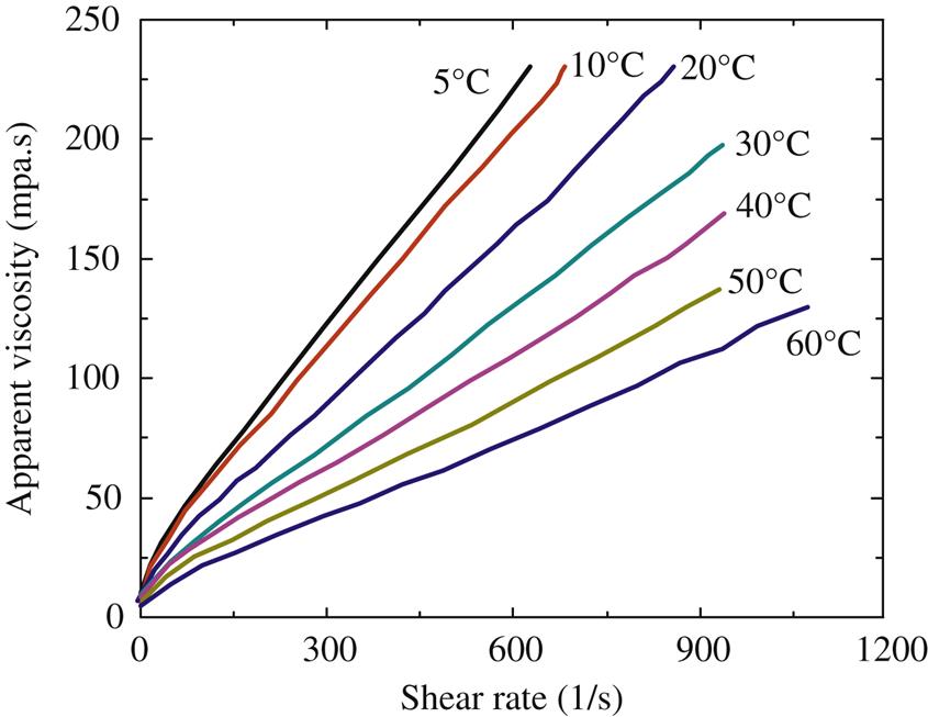
MR fluid directly dominates the property of MR dampers, and thus the fine rheological effect, antisettlement characteristics, and high magnetic saturation intensity are expected for MR fluid. In recent 20 years, Xu’s research group [229] developed many MR fluids, which have fine antisettlement characteristics and low apparent viscosity in low frequency vibration environment. Properties of a representative MR fluid are listed in Table 5.1. Fig. 5.1 shows the apparent viscosity curves under different temperatures, and Fig. 5.2 shows the yield shear stress with respect to magnetic induction intensity.

Table 5.1

Performance parameters of MR fluid

Type	MRFXZD08-01
Density (g/ml)	3.09
Solid content (%)	81.24
Flash point	>250°C
Apparent viscosity (30°C,500/s)	240 mPa·s
Operating temperature	−40–180°C
Coefficient of thermal expansion	3.4×10−4(1/°C)
Specific heat	1.36×105 J/(kg°C)
Magnetic saturation yield strength (1.0 T)	35 kPa

Magnetic core in the magnetic circuit is used to increase magnetic induction, change the magnetic flux intensity, and reduce magnetic flux leakage. The materials usually used for magnetic core are electrical pure iron, iron–nickel alloy, iron–aluminum alloy, soft magnetic ferrite, and so on. Compared with the traditional dampers, the material of MR dampers should meet the requirement of mechanical properties as well as good permeability performance. The material for magnetic core should consider the following items.

High magnetic permeability, it will produce high magnetic induction intensity when only small current is inputted.

The area of magnetic hysteretic loop should be small, the coercive force and the magnetic hysteresis loss should be small.

Good demagnetization ability, the magnetic field should quickly reduce to zero when the current is withdrawn.

The MR damper used in civil engineering structures consists of cylinder, piston, and the damping channel. The saturation induction density of the cylinder and piston should be higher than the magnetic field intensity of the MR fluid achieving magnetic saturation yield strength, so that the MR fluid can be fully utilized. What is more, the two parts are not only the parts of magnetic circuit, but also the main force delivery members of MR dampers. Therefore DT4 electrical pure iron and No. 45 steel, which have high magnetic permeability and high saturation induction density, are adopted for manufacturing the piston and the cylinder, respectively, whose B–H curves can be seen in Fig. 5.3. It can be seen that the saturation induction densities of the DT4 electrical pure iron and No. 45 steel are higher than the magnetic field intensity when MR fluid achieves magnetic saturation yield strength, this shows that the selected materials are meeting the requirements of the goals.

The resistance and reactance of the coil directly dominate the quantity of current, and the reactance of the coil is also related to the reluctance of the magnetic circuit. In terms of excitation coil, the following items should be considered.

The coil should avoid being too hot or even destroyed under the maximum current.

Determine the turns of the coil according to the nominal diameter and section diameter of the coil.

The coil should not have leakage electricity caused by the motion of the piston or abrasion of the coil.

5.1.1.2 Design principle

When designing a MR damper, the controllable force and the dynamic range are usually two of the most important parameters in evaluating the overall performance of MR dampers [230,231]. The total damping force $F$ produced by the shear-valve mode MR damper contains a controllable damping force $F_{\tau }$, a plastic viscous force $F_{\eta }$, and a friction force $F_f$ [232], as shown in Fig. 5.4.

$F=F_{\tau }+F_{\eta }+F_f$ (5.1)

(5.1)

In which, according to the parallel-plate Bingham model [233]

$F_{\tau }=\left(2.07+\frac{12Q\eta }{12Q\eta +0.4w{h}^2{\tau }_y}\right)\frac{{\tau }_{y}L{A}_p}{h}\mathrm{sgn}(v_0).$ (5.2)

(5.2)

$F_{\eta }=\left(1+\frac{wh{v}_0}{2Q}\right)\frac{12\eta Q{L}_t{A}_p}{w{h}^3}.$ (5.3)

(5.3)

where $L=L_1+L_2$ is the effective axial pole length. $L_t=L_1+L_2+L_3$ is the total axial pole length. $w$ is the mean circumference of the damper’s annular flow path $w=\pi (h/2+D+h/2)$, and $D$ is the diameter of the piston head. $h$ is the height of the annular flow path between piston and cylinder. $\eta$ and ${\tau }_y$ are the apparent viscosity without magnetic field and the yield shear strength of the MR fluid. $A_p$ is the effective cross-sectional area of the piston head $A_p=\pi (D^2-d_0^2)/4$, and $d_0$ is the diameter of the piston guide rod. $Q$ is the volumetric flow rate $Q=v_0\cdot A_p$. $v_0$ is the relative velocity between piston and cylinder, and sign function is used to consider the reciprocating of the piston.

According to Eq. (5.1), the total damping force can be decomposed into a controllable force $F_{\tau }$ and an uncontrollable force $F_{uc}=(F_{uc}=F_{\eta }+F_f)$. The uncontrollable force includes a plastic viscous force $F_{\eta }$ and a mechanical friction force $F_f$. The dynamic range $K$ is defined as the ratio between the controllable damping force $F_{\tau }$ and the uncontrollable force $F_{uc}$. If assume that $F_f=0$, then

$K=\frac{F_{\tau }}{F_{uc}}=\frac{F_{\tau }}{F_{\eta }+F_f}=\frac{F_{\tau }}{F_{\eta }}.$ (5.4)

(5.4)

For a given shock absorption application engineering, the dynamic range $K$ and the controllable damping force $F_{\tau }$ of MR dampers should be as large as possible, so that the designed MR damper can provide the engineering structure with the necessary damping force.

5.1.1.4 Magnetic circuit design

Magnetic circuit design is another important step to design a MR damper, magnetic circuit ohm's law is the basic formula to compute the magnetic induction intensity, and it is the basic principle for designing electromagnetic devices.

Usually, the magnetic circuit of the MR damper can be simplified as shown in Fig. 5.5. $g$ is the air gap length. According to the magnetic circuit ohm's law, the following equation can be obtained.

$NI=\mathrm{\Phi }(R_g+R_f)=\mathrm{\Phi }\left(\frac{l_1}{{\mu }_g{A}_g}+\frac{g}{{\mu }_f{A}_f}\right)$ (5.5)

(5.5)

where $R_g$ and $R_f$ are the magnetic reluctance of the magnetic core and air gap. The magnetic motive force is mainly used to overcome the magnetic reluctance of the air gap due to that the air gap has a large magnetic reluctance and small magnetic permeability, while the magnetic coil has large magnetic permeability and small magnetic reluctance. Thus the length of the air gap should be small as far as possible.

The objective of magnetic circuit design is to determine the number of the coils, so that the magnetic induction density in the annular flow path generated by magnetic circuit is larger than the magnetic saturation yield strength of MR fluid.

5.1.2 Parameters Optimization on MR Damper

The parameters optimization on MR damper includes two parts. One is the geometric optimization, and the other is the magnetic circuit optimization. Based on the discussion in Section 5.1.1, the optimization process will be introduced as follows.

5.1.2.1 Geometric optimization

The geometry of the MR damper depicted in Fig. 5.4 is designed considering engineering and test requirements, the maximum stroke and the required damping force of the MR damper are predetermined as 50 mm and 200 KN. The objective in designing the damper is to obtain a larger dynamic range $K$ with the damping force of 200 KN at the velocity of 100 mm/s. Therefore the geometry design process becomes the optimization problem of a constrained nonlinear multivariable function. The objective function, constraint condition, and design variables are as follows:

Object function: A larger dynamic range $K>15$.

Constraint condition: Total damping force $F=200\mathrm{KN}$ at the velocity of 100 mm/s.

Design variables: Diameter of the piston head $D$, diameter of the piston rod $d_0$, effective axial pole length $L$, total axial pole length $L_t$, and gap size $h$.

According to the objective function and constraint condition, the problem has been solved by properly adjusting the design variables using the function of fmincon in MATLAB. In this investigation, the designed variables are determined as $D=156\mathrm{mm}$, $d_0=80\mathrm{mm}$, $L=4\times L_1+2\times L_2=4\times 50+2\times 25=250\mathrm{mm}$, $L_t=500\mathrm{mm}$, and $h=2\mathrm{mm}$. In addition, main geometric parameters of the MR damper are shown in Table 5.2. Substituting the parameters into Eqs. (5.1)– (5.4), then

$\begin{array}{lll}{F}_{\tau }\hfill & =\hfill & \left(2.07+\frac{12Q\eta }{12Q\eta +0.4w{h}^2{\tau }_y}\right)\frac{{\tau }_{y}L{A}_p}{h}\hfill \\ \hfill & =\hfill & \left(2.07+\frac{12\times 0.00141\times 0.24}{12\times 0.00141\times 0.24+0.4\times 0.49\times {0.002}^2\times 35}\right)\times \frac{35\times 0.25\times 0.0141}{0.002}\hfill \\ \hfill & =\hfill & 188.97\mathrm{KN}\hfill \end{array}$ (5.6)

(5.6)

$\begin{array}{lll}{F}_{\eta }\hfill & =\hfill & \left(1+\frac{wh{v}_0}{2Q}\right)\frac{12\eta Q{L}_t{A}_p}{w{h}^3}\hfill \\ \hfill & =\hfill & \left(1+\frac{0.49\times 0.002\times 0.1}{2\times 0.00141}\right)\times \frac{12\times 0.24\times 0.00141\times 0.5\times 0.0141}{0.49\times {0.002}^3}\hfill \\ \hfill & =\hfill & 7.56\mathrm{KN}\hfill \end{array}$ (5.7)

(5.7)

$F=F_{\tau }+F_{\eta }=188.97+7.56=196.53\mathrm{KN}$ (5.8)

(5.8)

$K=\frac{F_{\tau }}{F_{\eta }}=\frac{188.97}{7.56}=25$ (5.9)

(5.9)

Table 5.2

Main geometric parameters of MR damper

Stroke (mm)	±50
External diameter of cylinder (mm)	194
Internal diameter of cylinder (mm)	160
Diameter of the piston rod (mm)	80
Effective length of the piston (mm)	4×50+2×25=250
Damping gap (mm)	2
Trench diameter of coil (mm)	110

As a result, the dynamic range is 25, the controllable damping force $F_{\tau }$ is 189 KN and the maximum damping force is 197 KN, these parameters can satisfy the design requirements completely.

5.1.2.2 Magnetic circuit optimization

Magnetic circuit directly determines the size of the magnetic induction density in the annular flow path. An optimal design of the magnetic circuit is required to maximize magnetic induction density in the annular flow path and minimize the energy loss in steel flux conduct and regions of nonworking areas. Here only one magnetic circuit will be designed because each stage of the magnetic circuit structure is the same as shown in Fig. 5.6.

According to Ohm's law [234], the following equation can be obtained

$NI=\mathrm{\Phi }\cdot (R_h+R_f)$ (5.10)

(5.10)

where $\Phi$ is the magnetic flux, $R_f$ and $R_h$ are the total iron core reluctance and annular flow path reluctance, respectively. $I$ is the current, $N$ is the number of the coils, $N=m\times n$, $m$ is the layer of the coil, $n$ and $d_w$ are the number of the coils at each layer and the diameter of the wire, respectively, as shown in Fig. 5.6.

Because magnetic circuit consists mainly of magnetic core, yoke, out cylinder, and annular flow path, the total iron core magnetic reluctance $R_f$ is considered to be composed of magnetic core reluctance $R_1$, yoke reluctance $R_2$, and cylinder reluctance $R_3$. The relative permeability of No. 45 steel (${\mu }_{\mathrm{s}\mathrm{t}\mathrm{e}\mathrm{e}\mathrm{l}}$), MR fluid (${\mu }_{\mathrm{M}\mathrm{R}\mathrm{F}}$), electrical pure iron DT4 (${\mu }_{\mathrm{i}\mathrm{r}\mathrm{o}\mathrm{n}}$), and copper wire (${\mu }_{\mathrm{c}\mathrm{o}\mathrm{i}\mathrm{l}}$) are 1000, 4, 1600, and 1, respectively. Then, considering the geometric parameters that have been determined in the geometry design, the magnetic reluctance $R_1$, $R_2$, $R_3$, and $R_h$ can be calculated according to Ohm's law and the pole surface of concentric cylinders gap permeance formula.

$R_1=\frac{4(L_1+L_2)}{\pi {\mu }_{\mathrm{s}\mathrm{t}\mathrm{e}\mathrm{e}\mathrm{l}}{d}^2}=\frac{4\times (0.05+0.025)}{\pi \times 1600\times 4\pi \times {10}^{-7}\times {0.11}^2}=3.93\times {10}^3$ (5.11)

(5.11)

$R_2=\frac{\ln (D/d)}{2\pi {\mu }_{\mathrm{i}\mathrm{r}\mathrm{o}\mathrm{n}}{L}_2}=\frac{\ln (0.156/0.11)}{2\pi \times 1600\times 4\pi \times {10}^{-7}\times 0.025}=1.11\times {10}^3$ (5.12)

(5.12)

$R_3=\frac{4(L_1+L_2)}{\pi {\mu }_{\mathrm{s}\mathrm{t}\mathrm{e}\mathrm{e}\mathrm{l}}(D_2^2-D_1^2)}=\frac{4\times (0.05+0.025)}{\pi \times 1000\times 4\pi \times {10}^{-7}\times ({0.194}^2-{0.16}^2)}=6.31\times {10}^3$ (5.13)

(5.13)

$R_h=\frac{\ln (D_1/D)}{2\pi {\mu }_{\mathrm{M}\mathrm{R}\mathrm{F}}{L}_2}=\frac{\ln (0.16/0.156)}{2\pi \times 4\times 4\pi \times {10}^{-7}\times 0.025}=3.21\times {10}^4$ (5.14)

(5.14)

Then, the total magnetic reluctance is calculated by the following equations

$R_m=R_1+2R_2+R_3+2R_h=7.666\times {10}^4$ (5.15)

(5.15)

According to magnetic saturation yield strength of MR fluid, take 1.0 T as the design value of the magnetic induction density in the annular flow path, then the magnetic flux in the magnetic circuit can be calculated as follows:

$\mathrm{\Phi }=B\times S=1.0\times \pi \times \left(\frac{0.160+0.156}{2}\right)\times 0.025=0.0124$ (5.16)

(5.16)

From Eq. (5.10), the current can be estimated as follows:

$I=\frac{\mathrm{\Phi }\cdot (R_h+R_f)}{N}=\frac{\mathrm{\Phi }\cdot R_m}{N}$ (5.17)

(5.17)

Then, the optimization problem with the magnetic circuit design is converted into searching for the design variables of a constrained nonlinear multivariable function. The objective function, constraint condition, and design variables are as follows:

Object function: $I\le 3$ A (maximum current of the direct current power supply).

Constraint condition: $NI\ge \mathrm{\Phi }\cdot R_m=0.0124\times 7.666\times {10}^4=950\mathrm{AT}$, $L_3\ge n\times d_w$, $\frac{D-d}{2}\ge m\times d_w$.

Design variables: $m$ is the layer of the coil, $n$ is the number of the coil at every layer, and $d_w$ is the diameter of the coil.

The problem can be solved by properly adjusting the design variables according to the objective function and the constraint conditions by using the function of fmincon in MATLAB. In this paper, the designed variables are $m=20$, $n=42$, $d_w=1.0\mathrm{mm}$, and the corresponding variables are $N=m\times n=840$, $I=1.13\mathrm{A}$, $L_3=50\ge 42\times 1=42$, $\frac{D-d}{2}=\frac{156-110}{2}=23\ge m\times d_w=20\times 1=20$.

Based on the above design and optimization process, the MR damper is manufactured and assembled according to the results of geometry design and magnetic circuit design, as shown in Fig. 5.7.

5.2.1 Parameters Optimization for Magnetic Circuit

For the MRE device introduced in Section 4.7.5 [210], the geometry configuration parameters of the magnetic circuit structure of the designed MRE device are shown in Fig. 5.8. The aim of parameter design is to design a magnetic circuit with low magnetic resistance, which can make the magnetic flux focus on the MRE working zone and avoid leakage flux occurring in other zones. The magnetic circuit consists of magnetic core (piston) and magnetic yoke (sleeve), so the magnetic resistance of each part should be calculated, which relates to the size of the member.

Based on the Ohm's law, the relationship between magnetic flux $\mathrm{\Phi }$ and magneto-motive F can be expressed as

$\mathrm{\Phi }=\frac{F}{R_m}$ (5.18)

(5.18)

$F=NI$ (5.19)

(5.19)

$\mathrm{\Phi }={\int }_{S}B\mathrm{d}S$ (5.20)

(5.20)

$R_m=\frac{l}{{\mu }_0\mu S}$ (5.21)

(5.21)

where R_m is magnetic resistance, N is number of coil cycles, I is field current, B is magnetic flux density, S is the area of the magnetic circuit, l is the length of the magnetic circuit, and $\mu$ is relative permeability. But for the specific calculation, the magnetic circuit can be simplified and shown in Fig. 5.9. Then, combined with the concentric cylindrical surface gap permanence formulas, the magnetic resistance of magnetic core, magnetic yoke, sleeve, and MRE can be calculated.

The magnetic resistance R_m1, R_m2, and R_m3 of magnetic core can be expressed as

$R_{m1}=\frac{l_1}{{\mu }_0{\mu }_1{S}_1}=\frac{4(h_1+h_2)}{{\mu }_0{\mu }_1\pi d^2}$ (5.22)

(5.22)

$R_{m2}=R_{m3}={\int }_d^D\frac{1}{2\pi {\mu }_0{\mu }_2{l}_2{h}_2}\mathrm{d}l=\frac{\ln (D/d)}{2\pi {\mu }_0{\mu }_2{h}_2}$ (5.23)

(5.23)

The magnetic resistance R_m4 of sleeve can be expressed as

$R_{m4}=\frac{l_4}{{\mu }_0{\mu }_4{S}_4}=\frac{4(h_1+h_2)}{{\mu }_0{\mu }_4\pi (D_2^2-D_1^2)}$ (5.24)

(5.24)

The magnetic resistance R_m5 and R_m6 can be expressed as

$R_{m5}=R_{m6}=\frac{l_5}{{\mu }_0{\mu }_5{S}_5}=\frac{\ln (D_1/D)}{2{\mu }_0{\mu }_5\pi h_2}$ (5.25)

(5.25)

The magnetic resistance R_m of the whole magnetic circuit can be expressed as

$R_m=R_{m1}+2R_{m2}+R_{m4}+2R_{m5}$ (5.26)

(5.26)

Here, the relative permeability of these magnetic materials of the MRE device can be got from the manufacturer, ${\mu }_{\mathrm{s}\mathrm{t}\mathrm{e}\mathrm{e}\mathrm{l}}=1000$ (the No. 45 steel), ${\mu }_{\mathrm{i}\mathrm{r}\mathrm{o}\mathrm{n}}=1600$ (DT₄ electric pure iron), ${\mu }_{\mathrm{c}\mathrm{o}\mathrm{i}\mathrm{l}}=1$ (copper interconnects), and the permeability of vacuum is ${\mu }_0=4\pi \times {10}^{-7}\mathrm{Wb}/\mathrm{A}\cdot \mathrm{m}$. However, the relative permeability of MRE cannot be given directly, so the important work is to analyze the permeability of MRE.

It can be seen in the references [60–62] that MRE is fabricated with the mixture of carbonyl iron powder particles and rubber-like elastomers, and theoretical analysis method is difficult to compute the relative permeability due to the nonlinear characteristics. Thus the electromagnetic finite element analysis method is used to simulate the magnetic field distribution under uniform magnetic field and calculate the relative permeability of MRE. One particle with the surrounded elastomers is detached as an element body which is shown in Fig. 5.10. The finite element model of the element body is built with the software ANSOFT Maxwell and the half section of the model along the cylinder axis is shown in Fig. 5.11.

Under the uniform magnetic field, the magnetic induction intensity distribution and magnetic force line distribution are calculated and shown in Fig. 5.12.

The relative permeability usually can be calculated by Eq. (5.27), where B₀ and H₀ separately are the average magnetic field intensity and the average magnetic induction intensity, respectively, which can be calculated by Eqs. (5.28) and (5.29). Therefore the calculated relative permeability of MRE can be obtained when the particles reach saturated magnetic intensity, which is about $u_r=2.34$.

${\mu }_r=\frac{B_0}{{\mu }_0{H}_0}$ (5.27)

(5.27)

$H_0=\sum _{i=1}^n{H}_{z,i}{V}_i/\sum _{i=1}^n{V}_i$ (5.28)

(5.28)

$B_0=\sum _{i=1}^n{B}_{z,i}{V}_i/\sum _{i=1}^n{V}_i$ (5.29)

(5.29)

According to the magnetic flux conservation law, the magnetic circuit magnetic flux of all parts should be equal, i.e., ${\mathrm{\Phi }}_1={\mathrm{\Phi }}_2={\mathrm{\Phi }}_3={\mathrm{\Phi }}_4={\mathrm{\Phi }}_5={\mathrm{\Phi }}_6$. The magnetic induction intensity can be calculated by $\mathrm{\Phi }=B\cdot S$. So, according to the relationship between the size of each part of the magnetic circuit and magnetic resistance, in order to get better utilization of the magnetic circuit by optimizing the parameters, each part of the magnetic circuit should reach magnetic saturation one after another, and the difference of the magnetic induction intensity at magnetic saturation between each part is small. Based on the above principle, the size of each part of the magnetic circuit can be optimized, and the optimization result is as follows: $d=38\mathrm{mm}$, $D=58\mathrm{mm}$, $D_1=70\mathrm{mm}$, $D_2=82\mathrm{mm}$, $h=6\mathrm{mm}$, $h_1=100\mathrm{mm}$, $h_2=10\mathrm{mm}$, and $D/d\approx 1.53$, $h_1/d\approx 2.11$, $(D_2-D_1)/2(h_1+h_2)\approx 0.055$. Substituting the above parameters into Eqs. (5.18)– (5.26), the magnetic induction intensity of each part of the magnetic circuit can be calculated and shown in Table 5.3.

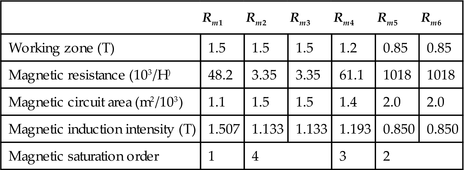
It can be seen from Table 5.3 that when the MRE working zone reaches magnetic saturation, the other parts of the magnetic circuit basically reach magnetic saturation, which demonstrates that the design of the whole magnetic circuit is reasonable.

5.2.2 Magnetic Circuit FEM Simulation

It is very difficult to get the accurate analytical solution for complex magnetic circuit structures, while some numerical methods, such as Finite Element Method (FEM), are commonly used to solve this problem. Therefore the software ANSOFT Maxwell is chosen to analyze the magnetic field distribution of the MRE device.

According to Section 5.2.2, the finite element model of the MRE device is built and shown in Fig. 5.13, and the calculating result is shown in Fig. 5.14. It can be seen that the magnetic induction of the iron core is about 1.25–1.56 T, the sleeve is about 1.04–1.38 T and the MRE is about 0.53–0.73 T, which is lower than the calculation results. The reason is that the B–H curve of materials is considered to be nonlinear in finite analysis but linear in the theoretical calculation. So the parameters should be adjusted to be in coincidence with the actual materials. Finally, the sizes of the iron core and sleeve are changed as:$d=48\mathrm{mm}$, $D=68\mathrm{mm}$, $D_1=80\mathrm{mm}$, and $D_2=96\mathrm{mm}$. The FEM model is rebuilt according to the changed parameters, and the analysis results are shown in Fig. 5.15.

It can be seen from Fig. 5.15 that the magnetic induction of iron core is about 1.32–1.65 T, the sleeve is about 1.1–1.32 T and the MRE is about 0.77–0.99 T, which are close to the calculation results. The detailed results of the two methods are shown in Table 5.4. It can be seen from Table 5.4 that the calculation results of the two methods match well, and there is a linear relationship between magnetic strength B and electric current I when the current is small (no more than 1.6 A). The above analysis results demonstrate that the magnetic circuit design of MRE device can be implemented with the simplified magnetic circuit method, which is based on the basic magnetic conductance theory. In other words, the simplified magnetic circuit method can be used for the preliminary design of MRE device. Then the FEM is used for further analysis of the magnetic circuit.

5.3.1 Design and Parameters Optimization Based on Feedback Gain

Sensors and actuators are typically placed on the position with the maximum structural vibration response, so the placement of sensors and actuators is not discussed. Nishimura et al. proposed a control strategy for AMD, the feedback gain and the AMD system parameters can be optimized simultaneously [235]. Neglecting the damping of the primary structure, Eqs. (3.3) and (3.4) can be rewritten as:

$m\ddot{x}(t)+kx(t)=p(t)+c_a{\stackrel{·}{x}}_a(t)+k_a{x}_a(t)-f_a(t)$ (5.30)

(5.30)

$m_a({\ddot{x}}_a(t)+\ddot{x}(t))+c_a{\stackrel{·}{x}}_a(t)+k_a{x}_a(t)=f_a(t)$ (5.31)

(5.31)

where $m_a{\ddot{x}}_a(t)$ is an active control force on the controlled structure, the control efficiency actually derived from the damping effect of tuned mass damper (TMD) on the primary structure and the output force of the actuator. The feedback gain of the proposed algorithm is linear to the response acceleration of the primal system, then the driving force can be expressed as

$f_a(t)=-G\ddot{x}(t)=-mg\ddot{x}(t)$ (5.32)

(5.32)

where $G$ is the feedback gain and $g$ is the normalized feedback gain. Introducing parameters $f=\frac{w}{w_0}$, $\beta =\frac{w_a}{w_0}$, $\mu =\frac{m_a}{m}$, and ${\xi }_a=\frac{c_a}{2m_a{w}_a}$, the frequency spectra response of the controlled structure is expressed as

${\left|H(f)\right|}^2=\frac{{({\beta }^2-f^2)}^2+{(2{\xi }_a\beta f)}^2}{{[(1-g)f^4-(1+{\beta }^2+\mu {\beta }^2)f^2+{\beta }^2]}^2+{[2{\xi }_a\beta f(1-f^2-\mu f^2)]}^2}$ (5.33)

(5.33)

The above response function of the controlled structure has two locked frequencies, where the corresponding responses are not influenced by the damping of the auxiliary mass. This phenomenon is similar to the case of TMD, so the optimization process of the TMD parameters can be conducted in the case of AMD. The final locked response value at the two locked points is given as

${\alpha }_{\max }=\sqrt{\frac{2+\mu -g_{\mathrm{o}\mathrm{p}\mathrm{t}}}{\mu +g_{\mathrm{o}\mathrm{p}\mathrm{t}}}}$ (5.34)

(5.34)

Hence the optimal feedback gain and the optimal frequency ratio are given as

$g_{\mathrm{o}\mathrm{p}\mathrm{t}}=\frac{2+\mu -\mu {\alpha }_{\max }^2}{{\alpha }_{\max }^2+1}$ (5.35)

(5.35)

${\beta }_{\mathrm{o}\mathrm{p}\mathrm{t}}=\sqrt{\frac{{\alpha }_{\max }^2-1}{(\mu +1)({\alpha }_{\max }^2+1)}}=\sqrt{\frac{1-g_{\mathrm{o}\mathrm{p}\mathrm{t}}}{1+\mu }}$ (5.36)

(5.36)

The damping of auxiliary mass determines the peak of the response function, and the optimal damping should satisfy the condition that the peaks appear under the locked points. The approximated value of the optimal damping is given by the corresponding equation in TMD, and the validity of the equation is checked by various combinations of the parameters.

${\xi }_{\mathrm{o}\mathrm{p}\mathrm{t}}=\sqrt{\frac{3}{4({\alpha }_{\max }^2+1)}}=\sqrt{\frac{3(\mu +g_{\mathrm{o}\mathrm{p}\mathrm{t}})}{8(1+\mu )}}$ (5.37)

(5.37)

When the control effect and the value of the auxiliary mass are given, then the value of ${\alpha }_{\max }$, the optimal feedback gain, the optimal frequency ratio and the optimal damping can be calculated. It can be found that the feedback belongs to acceleration feedback. Chang and Yang adopted velocity feedback and complete feedback to design and optimize the feedback gain and AMD system parameters [236].

5.3.2 Design and Parameters Optimization Based on Minimum Energy Principle

As mentioned in Section 3.2, the active control force applied to the structure is not equivalent to the driving force derived from the actuator. Based on the difference, Liu et al. proposed a design method of AMD control system, in which the active control force is determined firstly, and the next determination is about the driving force [237]. The equations of motion of the AMD control system can be expressed as

$\left[M\right]\{\ddot{x}(t)\}+\left[C\right]\{\stackrel{·}{x}(t)\}+\left[K\right]\{x(t)\}=\{P(t)\}+\left[B\right]\{f_d(t)\}$ (5.38)

(5.38)

$\{f_d(t)\}=\left[C_a\right]\{{\stackrel{·}{x}}_a(t)\}+\left[K_a\right]\{x_a(t)\}-\{f_a(t)\}=-\left[M_a\right]\{{\ddot{x}}_{aa}(t)\}$ (5.39)

(5.39)

where $\{f_d(t)\}$ is the active control force applied to the structure and $\{f_a(t)\}$ is the driving force derived from the actuator. In order to use active control algorithm to conduct the active control, Eq. (5.38) is rewritten as the state-space equation, and the performance index is defined as follows:

$J={\int }_0^{\infty }({(Z(t))}^{\mathrm{T}}[Q\left]\right\{Z(t)\}+{\{f_d(t)\}}^{\mathrm{T}}\eta [R\left]\right\{f_d(t)\})\mathrm{d}t.$ (5.40)

(5.40)

where $\eta$ is the weight coefficient that determines the control effect of structural vibration control, and the control force is calculated according to linear quadratic regulator (LQR) algorithm. In structural vibration control, the active control force is always written as the combination of the gain matrix and the structural state, then the driving force can be rewritten as

$\{f_a(t)\}=\left[C_a\right]\{{\stackrel{·}{x}}_a(t)\}+\left[K_a\right]\{x_a(t)\}+\left[G\right]\{Z(t)\}$ (5.41)

(5.41)

It can be seen from the above equation that the certain control effect must correspond to certain control force under a given active control algorithm. In other words, the provided control effect determines the control force, and the driving force is not determined due to the presence of AMD system parameters. The driving force can be calculated based on the relation between $\{f_d(t)\}$ and $\{f_a(t)\}$, but the selection of AMD system parameters is an important problem affecting the driving force. Obviously, the reasonable selection of parameters about AMD system can minimize the external input energy under a given vibration control effect, so the work done by the driving force is defined as the objective function

$\begin{array}{lll}J\hfill & =\hfill & {\int }_0^{t_f}(\{f_a(t)\left\}\right\{{\stackrel{·}{x}}_a(t)\})\mathrm{d}t\hfill \\ \hfill & =\hfill & {\int }_0^{t_f}((\left[C_a\right]\{{\stackrel{·}{x}}_a(t)\}+\left[K_a\right]\{x_a(t)\}+\left[G\right]\{Z(t)\})\{{\stackrel{·}{x}}_a(t)\})\mathrm{d}t\hfill \end{array}$ (5.42)

(5.42)

$x_a(t)={\int }_0^t{\int }_0^t(-{\left[M_a\right]}^{-1}\{f_d(\tau )\}-{\left[B\right]}^{\mathrm{T}}\{\ddot{x}(\tau )\})\mathrm{d}\tau \mathrm{d}\tau$ (5.43)

(5.43)

${\stackrel{·}{x}}_a(t)={\int }_0^t(-{\left[M_a\right]}^{-1}\{f_d(\tau )\}-{\left[B\right]}^{\mathrm{T}}\{\ddot{x}(\tau )\})\mathrm{d}\tau$ (5.44)

(5.44)

When the external excitation and the control effect are determined, the responses of the controlled structure and the active control force can be calculated. The basic parameters in objective function J are $\left[M_a\right]$, $\left[K_a\right]$, and $\left[C_a\right]$, which can be calculated by some numerical calculations. However, the selection of AMD system parameters is influenced by the external excitation, as a result the robustness is not good.

5.3.3 Design and Parameters Optimization Based on Fail-Safe Reliability

As described in Section 3.2, the design of control parameters of AMD control system is conducted after the optimization of the TMD parameters optimization, which can achieve a good control effect when the AMD fails to work or is not in a work state. For the parameters optimization of TMD, the mass of auxiliary mass can be determined according to the control effect and the practical engineering, the stiffness and damping of auxiliary mass can be obtained by the mature theoretical formula about optimal frequency ratio and damping ratio, such as the formula in Section 3.2 proposed by Tsai and Lin [73]. The driving force is calculated using active control algorithm, such as LQR algorithm described in Section 3.2.3.

It is worth noting that the weighting factors affect the control effect, the maximum driving force and the maximum stroke. The above indicators can be in a balanced state by optimizing the weighting factors. The detailed operation is to select reasonable performance index and define the range of parameters, such as stroke limits and maximum drive capability of AMD, then the numerical computation is adopted to calculate the reasonable weight factors.

$\left[Q\right]=\alpha \left[\begin{array}{cc}\left[K\right]& 0\\ 0& \left[M\right]\end{array}\right]\cdot \left[R\right]=\beta \left[I\right]$ (5.45)

(5.45)

where α and β are weighting factors. Although this design method has a high reliability of fail-safe, the control effect obtained is not optimal and economical, because the parameters are not based on global optimization.