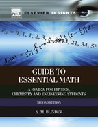
Matrix Algebra
Thus far, we have been doing algebra involving numbers and functions. It is also possible to apply the operations of algebra to more general types of mathematical entities. In this chapter, we will deal with matrices, which are ordered arrays of numbers or functions. For example, a matrix which we designate by the symbol ![]() can represent a collection of quantities arrayed as follows:
can represent a collection of quantities arrayed as follows:
 (9.1)
(9.1)
The subscripts ![]() and
and ![]() on the matrix elements
on the matrix elements![]() label the rows and columns, respectively. The matrix
label the rows and columns, respectively. The matrix ![]() shown above is an
shown above is an ![]() square matrix, with
square matrix, with ![]() rows and
rows and ![]() columns. We will also make use of
columns. We will also make use of ![]() column matrices or column vectors such as
column matrices or column vectors such as
 (9.2)
(9.2)
and ![]() row matrices or row vectors such as
row matrices or row vectors such as
![]() (9.3)
(9.3)
Where do matrices come from? Suppose we have a set of ![]() simultaneous relations, each involving
simultaneous relations, each involving ![]() quantities
quantities ![]() :
:
 (9.4)
(9.4)
This set of ![]() relations can be represented symbolically by a single matrix equation
relations can be represented symbolically by a single matrix equation
![]() (9.5)
(9.5)
where ![]() is the
is the ![]() matrix (9.1), while
matrix (9.1), while ![]() and
and ![]() are
are ![]() column vectors, such as (9.2).
column vectors, such as (9.2).
9.1 Matrix Multiplication
Comparing (9.4) with (9.5), it is seen that matrix multiplication implies the following rule involving their component elements:
![]() (9.6)
(9.6)
Note that summation over identical adjacent indices ![]() results in their mutual “annihilation.” Suppose the quantities
results in their mutual “annihilation.” Suppose the quantities ![]() in Eq. (9.4) are themselves determined by
in Eq. (9.4) are themselves determined by ![]() simultaneous relations
simultaneous relations
 (9.7)
(9.7)
The combined results of Eqs. (9.4) and (9.7), equivalent to eliminating ![]() between the two sets of equations, can be written
between the two sets of equations, can be written
 (9.8)
(9.8)
We can write the same equations in matrix notation:
![]() (9.9)
(9.9)
Evidently, ![]() can be represented as a matrix product:
can be represented as a matrix product:
![]() (9.10)
(9.10)
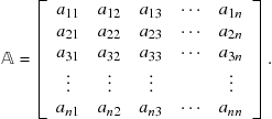
An element of the product matrix is constructed by summation over two sets of matrix elements in the following pattern:
![]() (9.11)
(9.11)
The diagram below shows schematically how the ijth element is constructed from the sum of products of elements from the ith row of the first matrix and the jth column of the second: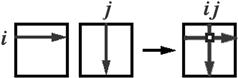
The three ![]() Pauli spin matrices
Pauli spin matrices
![]() (9.12)
(9.12)
will provide computationally simple examples to illustrate many of the properties of matrices. They are themselves of major significance in applications to quantum mechanics and geometry.
The most dramatic contrast between multiplication of matrices and multiplication of numbers is that matrix multiplication can be noncommutative, meaning that it is not necessarily true that
![]() (9.13)
(9.13)
As a simple illustration, consider products of Pauli spin matrices: We find
![]() (9.14)
(9.14)
also
![]() (9.15)
(9.15)
Matrix multiplication remains associative, however, so that
![]() (9.16)
(9.16)
In matrix multiplication, the product of an ![]() matrix and an
matrix and an ![]() matrix is an
matrix is an ![]() matrix. Two matrices cannot be multiplied unless their adjacent dimensions—
matrix. Two matrices cannot be multiplied unless their adjacent dimensions—![]() in the above example—match. As we have seen above, square matrix multiplying a column vector gives another column vector (
in the above example—match. As we have seen above, square matrix multiplying a column vector gives another column vector (![]() ). The product of a row vector and a column vector is an ordinary number (in a sense, a
). The product of a row vector and a column vector is an ordinary number (in a sense, a ![]() matrix). For example,
matrix). For example,
![]() (9.17)
(9.17)
Problem 9.1.1
Calculate and compare the matrix products ![]() and
and ![]() .
.
Problem 9.1.2
The commutator of two matrices is defined by
![]()
and the anticommutator by
![]()
Calculate the commutators and anticommutators for each pair of Pauli matrices.
9.2 Further Properties of Matrices
Following are a few hints on how to manipulate indices in matrix elements. It is most important to recognize that any index that is summed over is a dummy index. The result is independent of what we call it. Thus
![]() (9.18)
(9.18)
Secondly, it is advisable to use different indices when a product of summations occurs in an expression. For example,
![]()
This becomes mandatory if we reexpress it as a double summation
![]()
Multiplication of a matrix ![]() by a constant
by a constant ![]() is equivalent to multiplying each
is equivalent to multiplying each ![]() by
by ![]() . Two matrices of the same dimension can be added element by element. By combination of these two operations, the matrix elements of
. Two matrices of the same dimension can be added element by element. By combination of these two operations, the matrix elements of ![]() are given by
are given by ![]() .
.
The null matrix has all its elements equal to zero:
 (9.19)
As expected,
![]() (9.20)
(9.20)
A diagonal matrix has only nonvanishing elements along the main diagonal, for example
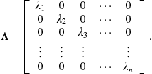 (9.21)
Its elements can be written in terms of the Kronecker delta:
![]() (9.22)
(9.22)
A diagonal matrix is sometimes represented in a form such as
![]() (9.23)
(9.23)
A special case is the unit or identity matrix, diagonal with all elements equal to 1:
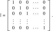 (9.24)
Clearly,
![]() (9.25)
(9.25)
As expected, for an arbitrary matrix ![]() :
:
![]() (9.26)
(9.26)
9.3 Determinants
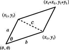
Determinants, an important adjunct to matrices, can be introduced as a geometrical construct. Consider the parallelogram shown in Figure 9.1, with one vertex at the origin ![]() and the other three at
and the other three at ![]() ,
, ![]() , and
, and ![]() . Using Pythagoras’ theorem, the two sides
. Using Pythagoras’ theorem, the two sides ![]() and the diagonal
and the diagonal ![]() have the lengths
have the lengths
![]() (9.27)
(9.27)
The area of the parallelogram is given by
![]() (9.28)
(9.28)
where ![]() is the angle between sides
is the angle between sides ![]() and
and ![]() . The
. The ![]() sign is determined by the relative orientation of
sign is determined by the relative orientation of ![]() and
and ![]() . Also, by the law of cosines,
. Also, by the law of cosines,
![]() (9.29)
(9.29)
Eliminating ![]() between Eqs. (9.28) and (9.29), we find, after some lengthy algebra, that
between Eqs. (9.28) and (9.29), we find, after some lengthy algebra, that
![]() (9.30)
(9.30)
(If you know about the cross product of vectors, this follows directly from ![]() .) This combination of variables has the form of a determinant, written
.) This combination of variables has the form of a determinant, written
![]() (9.31)
(9.31)
In general for a ![]() matrix
matrix ![]()
![]() (9.32)
(9.32)
The three-dimensional analog of a parallelogram is a parallelepiped, with all six faces being parallelograms. As shown in Figure 9.2, the parallelepiped is oriented between the origin ![]() and the point
and the point ![]() , which is the reflection of the origin through the plane containing the points
, which is the reflection of the origin through the plane containing the points ![]() , and
, and ![]() . You can figure out, using some algebra and trigonometry, that the volume is given by
. You can figure out, using some algebra and trigonometry, that the volume is given by
 (9.33)
[Using vector analysis, ![]() , where
, where ![]() are the vectors from the origin to
are the vectors from the origin to ![]() , respectively.]
, respectively.]
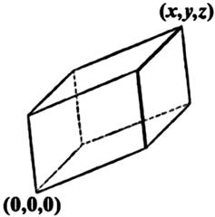
 .
.It might be conjectured that an ![]() -determinant represents the hypervolume of an
-determinant represents the hypervolume of an ![]() -dimensional hyperparallelepiped.
-dimensional hyperparallelepiped.
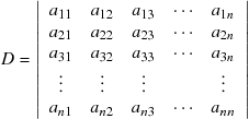
In general, a ![]() determinant is given by
determinant is given by
 (9.34)
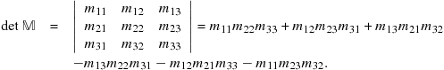
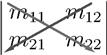
A ![]() determinant can be evaluated by summing over products of elements along the two diagonals, northwest-southeast minus northeast-southwest:
determinant can be evaluated by summing over products of elements along the two diagonals, northwest-southeast minus northeast-southwest:
Similarly for a ![]() determinant:
determinant:
 where the first two columns are duplicated on the right. There is no simple graphical method for
 ![]() or larger determinants. An
or larger determinants. An ![]() determinant is defined more generally by
determinant is defined more generally by
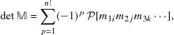 (9.35)
where ![]() is a permutation operator which runs over all
is a permutation operator which runs over all ![]() possible permutations of the indices
possible permutations of the indices ![]() The permutation label
The permutation label ![]() is even or odd, depending on the number of binary interchanges of the second indices necessary to obtain
is even or odd, depending on the number of binary interchanges of the second indices necessary to obtain ![]() , starting from its order on the main diagonal:
, starting from its order on the main diagonal: ![]() . Many math books show further reductions of determinants involving minors and cofactors, but this is no longer necessary with readily available computer programs to evaluate determinants. An important property of determinants, which is easy to verify in the
. Many math books show further reductions of determinants involving minors and cofactors, but this is no longer necessary with readily available computer programs to evaluate determinants. An important property of determinants, which is easy to verify in the ![]() and
and ![]() cases, is that if any two rows or columns of a determinant are interchanged, the value of the determinant is multiplied by
cases, is that if any two rows or columns of a determinant are interchanged, the value of the determinant is multiplied by ![]() . As a corollary, if any two rows or two columns are identical, the determinant equals zero.
. As a corollary, if any two rows or two columns are identical, the determinant equals zero.
The determinant of a product of two matrices, in either order, equals the product of their determinants. More generally for a product of three or more matrices, in any cyclic order,
![]() (9.36)
(9.36)
Problem 9.3.1
Find the volume of a unit cube coincident with the coordinate axes by evaluating a ![]() determinant.
determinant.
9.4 Matrix Inverse
The inverse of a matrix ![]() , designated
, designated ![]() , satisfies the matrix equation
, satisfies the matrix equation
![]() (9.37)
(9.37)
For the ![]() matrix
matrix
![]()
The inverse is given by
![]() (9.38)
(9.38)
For matrices of larger dimension, the inverses can be readily evaluated by computer programs. Note that the denominator in (9.38) equals the determinant of the matrix ![]() . In order for the inverse
. In order for the inverse ![]() to exist, the determinant of a matrix must not be equal to zero. Consequently, a matrix with determinant equal to zero is termed singular. A matrix with
to exist, the determinant of a matrix must not be equal to zero. Consequently, a matrix with determinant equal to zero is termed singular. A matrix with ![]() is called unimodular.
is called unimodular.
The inverse of a product of matrices equals the product of inverses in reversed order. For example,
![]() (9.39)
(9.39)
You can easily prove this by multiplying by ![]() .
.
The inverse matrix can be used to solve a series of simultaneous linear equations, such as (9.4). Supposing the ![]() are known quantities while the
are known quantities while the ![]() are unknowns, multiply the matrix equation (9.5) by
are unknowns, multiply the matrix equation (9.5) by ![]() . This gives
. This gives
![]() (9.40)
(9.40)
With the elements of ![]() and
and ![]() known, the column vector
known, the column vector ![]() , hence its elements
, hence its elements ![]() can be determined. The solutions are given explicitly by Cramer’s rule:
can be determined. The solutions are given explicitly by Cramer’s rule:
![]() (9.41)
(9.41)
where ![]() is the determinant of the matrix
is the determinant of the matrix ![]() :
:
 (9.42)
and ![]() is obtained from
is obtained from ![]() by replacing the ith column by the column vector
by replacing the ith column by the column vector ![]() :
:
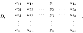 (9.43)
A set of homogeneous linear equations
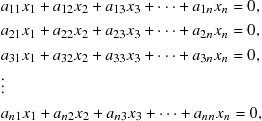 (9.44)
always has the trivial solution![]() . A necessary condition for a nontrivial solution to exist is that
. A necessary condition for a nontrivial solution to exist is that ![]() . (This is not a sufficient condition, however. The trivial solution might still be the only one.)
. (This is not a sufficient condition, however. The trivial solution might still be the only one.)
Problem 9.4.1
Find the inverses of the three Pauli matrices, ![]() , and
, and ![]() .
.
Problem 9.4.2
Using Cramer’s rule, solve the set of simultaneous linear equations

9.5 Wronskian Determinant
A set of ![]() functions
functions ![]() is said to be linearly independent if vanishing of the linear combination
is said to be linearly independent if vanishing of the linear combination
![]() (9.45)
(9.45)
can only be achieved with the “trivial” solution
![]()
A criterion for linear independence can be obtained by constructing a set of ![]() simultaneous equations involving (9.45) along with its 1st, 2nd, …, (n − 1)st derivatives:
simultaneous equations involving (9.45) along with its 1st, 2nd, …, (n − 1)st derivatives:
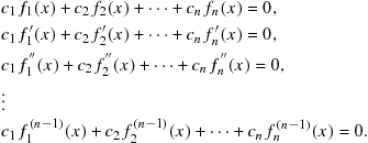 (9.46)
A trivial solution, hence linear independence, is guaranteed if the Wronskian determinant is nonvanishing, i.e.
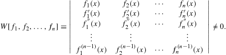 (9.47)
You can show, for example, that the set ![]() is linearly independent, while the set
is linearly independent, while the set ![]() is not.
is not.
Problem 9.5.1
Test the pair of functions ![]() for linear independence.
for linear independence.
Problem 9.5.2
Similarly test the set ![]() .
.
9.6 Special Matrices
The transpose of a matrix, designated ![]() or
or ![]() , is obtained by interchanging its rows and columns or, alternatively, by reflecting all the matrix elements through the main diagonal:
, is obtained by interchanging its rows and columns or, alternatively, by reflecting all the matrix elements through the main diagonal:
![]() (9.48)
(9.48)
A matrix equal to its transpose, ![]() , is called symmetric. Two examples of symmetric matrices are
, is called symmetric. Two examples of symmetric matrices are
![]() (9.49)
(9.49)
If ![]() , the matrix is skew-symmetric, for example
, the matrix is skew-symmetric, for example
![]() (9.50)
(9.50)
A matrix is orthogonal if its transpose equals its inverse: ![]() . A
. A ![]() unimodular orthogonal matrix—also known as a special orthogonal matrix—can be expressed in the form
unimodular orthogonal matrix—also known as a special orthogonal matrix—can be expressed in the form
![]() (9.51)
(9.51)
The totality of such two-dimensional matrices is known as the special orthogonal group, designated SO(2). The rotation of a Cartesian coordinate system in a plane, such that
![]() (9.52)
(9.52)
can be compactly represented by the matrix equation
![]() (9.53)
(9.53)
Since ![]() is orthogonal,
is orthogonal, ![]() , which leads to the invariance relation
, which leads to the invariance relation
![]() (9.54)
(9.54)
As a general principle, a linear transformation preserves length if and only if its matrix is orthogonal.
The Hermitian conjugate of a matrix, ![]() , is obtained by transposition accompanied by complex conjugation:
, is obtained by transposition accompanied by complex conjugation:
![]() (9.55)
(9.55)
A matrix is Hermitian or self-adjoint if ![]() . The matrices
. The matrices ![]() , and
, and ![]() introduced above are all Hermitian. The Hermitian conjugate of a product equals the product of conjugates in reverse order:
introduced above are all Hermitian. The Hermitian conjugate of a product equals the product of conjugates in reverse order:
![]() (9.56)
(9.56)
analogous to the inverse of a product. The same ordering is true for the transpose of a product. Also, it should be clear that a second Hermitian conjugation returns a matrix to its original form:
![]() (9.57)
(9.57)
The analogous effect of double application is also true for the inverse and the transpose. A matrix is unitary if its Hermitian conjugate equals its inverse: ![]() . The set of
. The set of ![]() unimodular unitary matrices constitutes the special unitary group SU(2). Such matrices can be parametrized by
unimodular unitary matrices constitutes the special unitary group SU(2). Such matrices can be parametrized by
![]() (9.58)
(9.58)
or by
![]() (9.59)
(9.59)
The SU(2) matrix group is of significance in the physics of spin-![]() particles.
particles.
9.7 Similarity Transformations
A matrix ![]() is said to undergo a similarity transformation to
is said to undergo a similarity transformation to ![]() if
if
![]() (9.60)
(9.60)
where the transformation matrix![]() is nonsingular. (The transformation is alternatively written
is nonsingular. (The transformation is alternatively written ![]() .) When the matrix
.) When the matrix ![]() is orthogonal, we have an orthogonal transformation:
is orthogonal, we have an orthogonal transformation: ![]() . When the transformation matrix is unitary, we have a unitary transformation:
. When the transformation matrix is unitary, we have a unitary transformation: ![]() . All similarity transformations preserve the form of matrix equations. Suppose
. All similarity transformations preserve the form of matrix equations. Suppose
![]()
Premultiplying by ![]() and postmultiplying by
and postmultiplying by ![]() , we have
, we have
![]()
Inserting ![]() in the form of
in the form of ![]() between
between ![]() and
and ![]() :
:
![]()
From the definition of primed matrices in Eq. (9.60), we conclude
![]() (9.61)
(9.61)
This is what we mean by the form of a matrix relation being preserved under a similarity transformation. The determinant of a matrix is also invariant under a similarity transformation, since
![]() (9.62)
(9.62)
9.8 Matrix Eigenvalue Problems
One important application of similarity transformations is to reduce a matrix to diagonal form. This is particularly relevant in quantum mechanics, when the matrix is Hermitian and the transformation unitary. Consider the relation
![]() (9.63)
(9.63)
where ![]() is a diagonal matrix, such as (9.21). Premultiplying by
is a diagonal matrix, such as (9.21). Premultiplying by ![]() , this becomes
, this becomes
![]() (9.64)
(9.64)
Expressed in terms of matrix elements:
![]() (9.65)
(9.65)
recalling that the elements of the diagonal matrix are given by ![]() and noting that only the term with
and noting that only the term with ![]() will survive the summation over
will survive the summation over ![]() . The unitary matrix
. The unitary matrix ![]() can be pictured as composed of an array of column vectors
can be pictured as composed of an array of column vectors ![]() , such that
, such that ![]() , like this:
, like this:
 (9.66)
Accordingly Eq. (9.64) can be written as a set of equations
![]() (9.67)
(9.67)
This is an instance of an eigenvalue equation. In general, a matrix ![]() operating on a vector
operating on a vector ![]() will produce another vector
will produce another vector ![]() , as shown in Eq. (9.5). For certain very special vectors
, as shown in Eq. (9.5). For certain very special vectors ![]() , the matrix multiplication miraculously reproduces the original vector multiplied by a constant
, the matrix multiplication miraculously reproduces the original vector multiplied by a constant ![]() , so that
, so that
![]() (9.68)
(9.68)
Eigenvalue problems are most frequently encountered in quantum mechanics. The differential equation for the particle-in-a-box, treated in Section 8.6, represents another type of eigenvalue problem. There, the boundary conditions restricted the allowed energy values to the discrete set ![]() , enumerated in Eq. (8.111). These are consequently called energy eigenvalues.
, enumerated in Eq. (8.111). These are consequently called energy eigenvalues.
The eigenvalues of a Hermitian matrix are real numbers. This follows by taking the Hermitian conjugate of Eq. (9.63):
![]() (9.69)
(9.69)
Since ![]() , by its Hermitian property, we conclude that
, by its Hermitian property, we conclude that
![]() (9.70)
(9.70)
Hermitian eigenvalues often represent physically observable quantities, consistent with their values being real numbers.
The eigenvalues and eigenvectors can be found by solving the set of simultaneous linear equations represented by (9.67):
 (9.71)
This reduces to a set of homogeneous equations:
 (9.72)
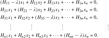
A necessary condition for a nontrivial solution is the vanishing of the determinant:
 (9.73)
this is known as the secular equation and can be solved for ![]() roots
roots ![]() .It is a general result that the eigenvectors of two unequal eigenvalues are orthogonal. To prove this, consider two different eigensolutions of a matrix
.It is a general result that the eigenvectors of two unequal eigenvalues are orthogonal. To prove this, consider two different eigensolutions of a matrix ![]() :
:
![]() (9.74)
(9.74)
Now, take the Hermitian conjugate of the ![]() equation, recalling that
equation, recalling that ![]() is Hermitian (
is Hermitian (![]() ) and
) and ![]() is real (
is real (![]() ). Thus
). Thus
![]() (9.75)
(9.75)
Now postmultiply the last equation by ![]() , premultiply the
, premultiply the ![]() equation by
equation by ![]() , and subtract the two. The result is
, and subtract the two. The result is
![]() (9.76)
(9.76)
If ![]() , then
, then ![]() and
and ![]() are orthogonal:
are orthogonal:
![]() (9.77)
(9.77)
When ![]() , although
, although ![]() , the proof fails. The two eigenvectors
, the proof fails. The two eigenvectors ![]() and
and ![]() are said to be degenerate. It is still possible to find a linear combination of
are said to be degenerate. It is still possible to find a linear combination of ![]() and
and ![]() so that the orthogonality relation Eq. (9.77) still applies. If, in addition, all the eigenvectors are normalized, meaning that
so that the orthogonality relation Eq. (9.77) still applies. If, in addition, all the eigenvectors are normalized, meaning that
![]() (9.78)
(9.78)
then the set of eigenvectors ![]() constitutes an orthonormal set satisfying the compact relation
constitutes an orthonormal set satisfying the compact relation
![]() (9.79)
(9.79)
analogous to the relation for orthonormalized eigenfunctions.
In quantum mechanics there is a very fundamental connection between matrices and integrals involving operators and their eigenfunctions. A matrix we denote as ![]() is defined such that its matrix elements correspond to integrals over an operator
is defined such that its matrix elements correspond to integrals over an operator ![]() and its eigenfunctions
and its eigenfunctions ![]() , constructed as follows:
, constructed as follows:
![]() (9.80)
(9.80)
The two original formulations of quantum mechanics were Heisenberg’s matrix mechanics (1925), based on representation of observables by noncommuting matrices and Schrödinger’s wave mechanics (1926), based on operators and differential equations. It was deduced soon afterward by Schrödinger and by Dirac that the two formulations were equivalent representations of the same underlying physical theory, a key connection being the equivalence between matrices and operators demonstrated above.
Problem 9.8.1
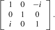
Find the eigenvalues and normalized eigenvectors for each of the three Pauli matrices, ![]() , and
, and ![]() .
.
Problem 9.8.2
Find the eigenvalues and normalized eigenvectors of the matrix
9.9 Diagonalization of Matrices
A matrix ![]() is diagonalizable if there exists a similarity transformation of the form
is diagonalizable if there exists a similarity transformation of the form
![]() (9.81)
(9.81)
All Hermitian, symmetric, unitary, and orthogonal matrices are diagonalizable, as is any ![]() -matrix whose
-matrix whose ![]() eigenvalues are distinct. The process of diagonalization is essentially equivalent to determination of the eigenvalues of a matrix, which are given by the diagonal elements
eigenvalues are distinct. The process of diagonalization is essentially equivalent to determination of the eigenvalues of a matrix, which are given by the diagonal elements ![]() .
.
The trace of a matrix is defined as the sum of its diagonal elements:
![]() (9.82)
(9.82)
This can be shown to be equal to the sum of its eigenvalues. Since
![]() (9.83)
(9.83)
we can write
![]() (9.84)
(9.84)
noting that ![]() . Therefore
. Therefore
![]() (9.85)
(9.85)
Problem 9.1.1
Find similarity transformations which diagonalize the Pauli matrices ![]() and
and ![]() .
.
9.10 Four-Vectors and Minkowski Spacetime
Suppose that at ![]() a light flashes at the origin, creating a spherical wave propagating outward at the speed of light
a light flashes at the origin, creating a spherical wave propagating outward at the speed of light ![]() . The locus of the wavefront will be given by
. The locus of the wavefront will be given by
![]() (9.86)
(9.86)
According to Einstein’s Special Theory of Relativity, the wave will retain its spherical appearance to every observer, even one moving at a significant fraction of the speed of light. This can be expressed mathematically as the invariance of the differential element
![]() (9.87)
(9.87)
known as the spacetime interval. Equation (9.87) has a form suggestive of Pythagoras’ theorem in four dimensions. It was fashionable in the early years of the 20th century to define an imaginary time variable ![]() , which together with the space variables
, which together with the space variables ![]() , and
, and ![]() forms a pseudo-Euclidean four-dimensional space with interval given by
forms a pseudo-Euclidean four-dimensional space with interval given by
![]() (9.88)
(9.88)
This contrived Euclidean geometry doesn’t change the reality that time is fundamentally very different from a spatial variable. It is current practice to accept the differing signs in the spacetime interval and define a real time variable ![]() , in terms of which
, in terms of which
![]() (9.89)
(9.89)
The corresponding geometrical structure is known as Minkowski spacetime. The form we have written, described as having the signature![]() , is preferred by elementary-particle physicists. People working in General Relativity write instead
, is preferred by elementary-particle physicists. People working in General Relativity write instead ![]() , with signature
, with signature ![]() .
.
The spacetime variables are the components of a Minkowski four-vector, which can be thought of as a column vector
 (9.90)
with its differential analog
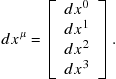 (9.91)
Specifically, these are contravariant four-vectors, with their component labels written as superscripts. The spacetime interval (9.89) can be represented as a scalar product if we define associated covariant four-vectors as the row matrices
![]() (9.92)
(9.92)
with the component indices written as subscripts. A matrix product can then be written:
 (9.93)
This accords with (9.89) provided that the covariant components ![]() are given by
are given by
![]() (9.94)
(9.94)
It is convenient to introduce the Einstein summation convention for products of covariant and contravariant vectors, whereby
 (9.95)
Any term containing the same Greek covariant and contravariant indices is understood to be summed over that index. This applies even to tensors, objects with multiple indices. For example, a valid tensor equation might read
![]() (9.96)
(9.96)
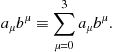
The equation applies for all values of the indices which are not summed over. The index ![]() summed from 0 to 3 is said to be contracted. Usually, the summation convention for Latin indices implies a sum just from 1 to 3, for example
summed from 0 to 3 is said to be contracted. Usually, the summation convention for Latin indices implies a sum just from 1 to 3, for example
![]() (9.97)
(9.97)
A four-dimensional scalar product can alternatively be written
![]() (9.98)
(9.98)
Covariant and contravariant vectors can be interconverted with use of the metric tensor![]() , given by
, given by
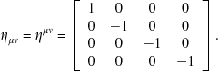 (9.99)
For example,
![]() (9.100)
(9.100)
The spacetime interval takes the form
![]() (9.101)
(9.101)
In General Relativity, the metric tensor ![]() is determined by the curvature of spacetime and the interval generalizes to
is determined by the curvature of spacetime and the interval generalizes to
![]() (9.102)
(9.102)
where ![]() might have some nonvanishing off-diagonal elements. In flat spacetime (in the absence of curvature), this reduces to Special Relativity with
might have some nonvanishing off-diagonal elements. In flat spacetime (in the absence of curvature), this reduces to Special Relativity with ![]() .
.
The energy and momentum of a particle in relativistic mechanics can also be represented as components of a four-vector ![]() with
with
![]() (9.103)
(9.103)
![]() (9.104)
(9.104)
The scalar product is an invariant quantity
![]() (9.105)
(9.105)
where ![]() is the rest mass of the particle. Written out explicitly, this gives the relativistic energy-momentum relation:
is the rest mass of the particle. Written out explicitly, this gives the relativistic energy-momentum relation:
![]() (9.106)
(9.106)
In the special case of a particle at rest ![]() , we obtain Einstein’s famous mass-energy equation
, we obtain Einstein’s famous mass-energy equation ![]() . The alternative root
. The alternative root ![]() is now understood to pertain to the corresponding antiparticle. For a particle with zero rest mass, such as the photon, we obtain
is now understood to pertain to the corresponding antiparticle. For a particle with zero rest mass, such as the photon, we obtain ![]() . Recalling that
. Recalling that ![]() , this last four-vector relation is consistent with both the Planck and de Broglie formulas:
, this last four-vector relation is consistent with both the Planck and de Broglie formulas: ![]() and
and ![]() .
.