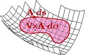
Vector Analysis
The perceptible physical world is three dimensional (although additional hidden dimensions have been speculated in superstring theories and the like). The most general mathematical representations of physical laws should therefore be relations involving three dimensions. Such equations can be compactly expressed in terms of vectors. Vector analysis is particularly applicable in formulating the laws of electromagnetic theory.
12.1 Scalars and Vectors
A scalar is a quantity which is completely described by its magnitude—a numerical value and usually a unit. Mass and temperature are scalars, with values, for example, like 10 kg and 300 K. A vector has, in addition, a direction. Velocity and force are vector quantities. A vector is usually printed as a boldface symbol, like ![]() , while a scalar is printed in normal weight, usually in italics, like a. (Vectors are commonly handwritten by placing an arrow over the symbol, like
, while a scalar is printed in normal weight, usually in italics, like a. (Vectors are commonly handwritten by placing an arrow over the symbol, like ![]() or
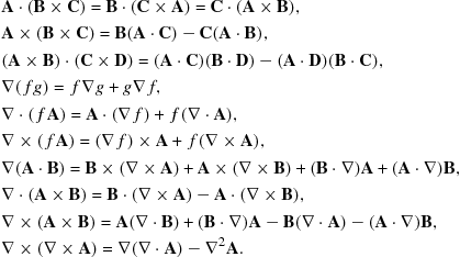
or ![]() .) A vector in three-dimensional space can be considered as a sum of three components. Figure 12.1 shows a vector
.) A vector in three-dimensional space can be considered as a sum of three components. Figure 12.1 shows a vector ![]() with its Cartesian components
with its Cartesian components ![]() , alternatively written
, alternatively written ![]() . The vector
. The vector ![]() is represented by the sum
is represented by the sum
![]() (12.1)
(12.1)
where i, j, k are unit vectors in the x, y, z directions, respectively. These are alternatively written ![]() or
or ![]() . The unit vectors have magnitude one and are directed along the positive x, y, z axes, respectively. They are pure numbers, so that the units of A are carried by the components
. The unit vectors have magnitude one and are directed along the positive x, y, z axes, respectively. They are pure numbers, so that the units of A are carried by the components ![]() . A vector can also be represented in matrix notation by
. A vector can also be represented in matrix notation by
![]() (12.2)
(12.2)
The magnitude of a vector A is written ![]() or A. By Pythagoras’ theorem in three dimensions we have
or A. By Pythagoras’ theorem in three dimensions we have
![]() (12.3)
(12.3)
Newton’s second law, written as a vector equation
![]() (12.4)
(12.4)
is shorthand for the three component relations
![]() (12.5)
(12.5)
Also (12.4) implies the corresponding relation between the scalar magnitudes
![]() (12.6)
(12.6)
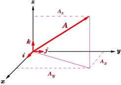
Figure 12.1 Vector A with Cartesian components ![]() . Unit vectors i, j, k are also shown. The length or magnitude of A is given by
. Unit vectors i, j, k are also shown. The length or magnitude of A is given by ![]() .
.
A significant mathematical property of vector relationships is their invariance under translation and rotation. For example, if F and a are transformed to ![]() and
and ![]() by translation and/or rotation, the analog of (12.4), namely
by translation and/or rotation, the analog of (12.4), namely
![]() (12.7)
(12.7)
along with all the corresponding component relationships, is also valid. Note that scalar quantities do not change under such transformations, so ![]() .
.
A vector can be multiplied by a scalar, such that
![]() (12.8)
(12.8)
For ![]() , this changes the magnitude of the vector while preserving its direction. For
, this changes the magnitude of the vector while preserving its direction. For ![]() , the direction of the vector is reversed. Two vectors can be added using
, the direction of the vector is reversed. Two vectors can be added using
![]() (12.9)
(12.9)
As shown in Figure 12.2, a vector sum can be obtained either by a parallelogram construction or by a triangle construction—placing the two vectors head to tail. Vectors can be moved around at will, so long as their magnitudes and directions are maintained. This is called parallel transport. (Parallel transport is easy in Euclidean space but more complicated in curved spaces such as the surface of a sphere. Here the vector must be moved in such a way that it maintains its orientation along geodesics. Parallel transport around a closed path in a non-Euclidean space usually changes the direction of a vector.)
The position or displacement vector r represents the three Cartesian coordinates of a point:
![]() (12.10)
(12.10)
A single symbol r can thus stand for the three coordinates ![]() in the same sense that a complex number z represents the pair of numbers
in the same sense that a complex number z represents the pair of numbers ![]() and
and ![]() . A unit vector in the direction of r can be written
. A unit vector in the direction of r can be written
![]() (12.11)
(12.11)
A differential element of displacement can likewise be defined by
![]() (12.12)
(12.12)
The notation ds is often used for a differential element of a curve in two- or three-dimensional space.
A function of x, y, and z can be compactly written
![]() (12.13)
(12.13)
If ![]() is a scalar, this represents a scalar field. If there is, in addition, dependence on another variable, such as time, we could write
is a scalar, this represents a scalar field. If there is, in addition, dependence on another variable, such as time, we could write ![]() . If the three components of a vector
. If the three components of a vector ![]() are functions of
are functions of ![]() , we have a vector field
, we have a vector field
![]() (12.14)
(12.14)
or A(r,t) if it is time dependent.
12.2 Scalar or Dot Product
Vectors can be multipled in two different ways to give scalar products and vector products. The scalar product, written ![]() , also called the dot product or the inner product, is equal to a scalar. To see where the scalar product comes from, recall that work in mechanics equals force times displacement. If the force and displacement are not in the same direction, only the component of force along the displacement produces work. We can write
, also called the dot product or the inner product, is equal to a scalar. To see where the scalar product comes from, recall that work in mechanics equals force times displacement. If the force and displacement are not in the same direction, only the component of force along the displacement produces work. We can write ![]() , where
, where ![]() is the angle between the vectors F and r.
is the angle between the vectors F and r.
We are thus led to define the scalar product of two vectors by
![]() (12.15)
(12.15)
When B = A, ![]() and
and ![]() , so the dot product reduces to the square of the magnitude of A:
, so the dot product reduces to the square of the magnitude of A:
![]() (12.16)
(12.16)
When A and B are orthogonal (perpendicular), ![]() and
and ![]() , so that
, so that
![]() (12.17)
(12.17)
The scalar products involving the three unit vectors are therefore given by
![]() (12.18)
(12.18)
These vectors thus constitute an orthonormal set with respect to scalar multiplication. To express the scalar product ![]() in terms of the components of A and B, write
in terms of the components of A and B, write
![]() (12.19)
(12.19)
Using (12.18) for the products of unit vectors, we find
![]() (12.20)
(12.20)
The scalar product has the same structure as the three-dimensional matrix product of a row vector with a column vector:
![]() (12.21)
(12.21)
12.3 Vector or Cross Product
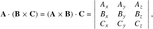
Consider a point P rotating counterclockwise about a vertical axis through the origin, as shown in Figure 12.3. Let r be the vector from the origin to point P and v, the instantaneous linear velocity of the point as it moves around a circle of radius ![]() . A rotation is conventionally represented by an axial vector
. A rotation is conventionally represented by an axial vector![]() normal to the plane of motion, such that the trajectory of P winds about
normal to the plane of motion, such that the trajectory of P winds about ![]() in a counterclockwise sense, the same as the direction a right-handed screw advances as it is turned. This is remembered most easily by using the right-hand rule shown in Figure 12.4. A rotational velocity of
in a counterclockwise sense, the same as the direction a right-handed screw advances as it is turned. This is remembered most easily by using the right-hand rule shown in Figure 12.4. A rotational velocity of ![]() radians/s moves point P with a speed
radians/s moves point P with a speed ![]() around the circle. The velocity vector v thus has magnitude
around the circle. The velocity vector v thus has magnitude ![]() and instantaneous direction normal to both r and
and instantaneous direction normal to both r and ![]() . This motivates definition of the vector product, also known as the cross product or the outer product, such that
. This motivates definition of the vector product, also known as the cross product or the outer product, such that
![]() (12.22)
(12.22)
The direction of v is determined by the counterclockwise rotation of the first vector ![]() into the second r, shown also in Figure 12.4.
into the second r, shown also in Figure 12.4.
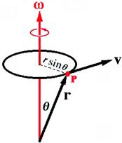
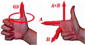
Figure 12.4 Right-hand rules. Left: Direction of axial vector ![]() representing counterclockwise rotation. Right: Direction of vector product
representing counterclockwise rotation. Right: Direction of vector product ![]() .
.
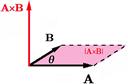
As another way to arrive at the vector product, consider the parallelogram with adjacent sides formed by vectors A and B, as shown in Figure 12.5. The area of the parallelogram is equal to its base A times its altitude ![]() . By definition, the vector product
. By definition, the vector product ![]() has magnitude
has magnitude ![]() and direction normal to the parallelogram. The operation of vector multiplication is anticommutative since
and direction normal to the parallelogram. The operation of vector multiplication is anticommutative since
![]() (12.23)
(12.23)
This implies that the cross product of a vector with itself equals zero:
![]() (12.24)
(12.24)
By contrast, scalar multiplication is commutative with
![]() (12.25)
(12.25)
The three unit vectors have the following vector products:
![]() (12.26)
(12.26)
Therefore, the cross product of two vectors in terms of their components can be determined from
![]() (12.27)
(12.27)
This can be compactly represented as a ![]() determinant:
determinant:
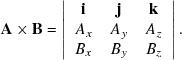 (12.28)
The individual components are given by
![]() (12.29)
(12.29)
where “et cyc” stands for the other two relations obtained by cyclic permutations ![]() . Another way to write a cross product is
. Another way to write a cross product is
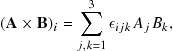 (12.30)
in terms of the Levi-Civita symbol![]() , defined by
, defined by
 (12.31)
The vector product occurs in the force law for a charged particle moving in an electromagnetic field. A particle with charge q moving with velocity v in an electric field E and a magnetic induction field B experiences a Lorentz force:
![]() (12.32)
(12.32)
The magnetic component of the force is perpendicular to both the velocity and the magnetic induction, which causes charged particles to deflect into curved paths. This underlies the principle of the cyclotron and other particle accelerators.
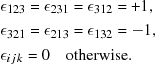
Inversion of a coordinate system means reversing the directions if the ![]() axes, or equivalently replacing
axes, or equivalently replacing ![]() by
by ![]() . This amounts to turning a right-handed into a left-handed coordinate system. A polar vector is transformed into its negative by inversion, as shown in Figure 12.6. A circulation in three dimensions, which can be represented by an axial vector, remains, by contrast, unchanged under inversion. An axial vector is also called a pseudovector to highlight its different inversion symmetry. The vector product of two polar vectors gives an axial vector: symbolically,
. This amounts to turning a right-handed into a left-handed coordinate system. A polar vector is transformed into its negative by inversion, as shown in Figure 12.6. A circulation in three dimensions, which can be represented by an axial vector, remains, by contrast, unchanged under inversion. An axial vector is also called a pseudovector to highlight its different inversion symmetry. The vector product of two polar vectors gives an axial vector: symbolically, ![]() . You can show also that
. You can show also that ![]() and
and ![]() . In electromagnetic theory, the electric field E is a polar vector while the magnetic induction B is an axial vector. This is consistent with the fact that magnetic fields originate from circulating electric charges.
. In electromagnetic theory, the electric field E is a polar vector while the magnetic induction B is an axial vector. This is consistent with the fact that magnetic fields originate from circulating electric charges.
Problem 12.3.1
A charged particle in an electromagnetic field is described by the Lagrangian
![]()
where q is the electric charge and ![]() , where A is the vector potential. As a generalization of the result of Problem 11.6.1, derive the corresponding Hamiltonian H(r, p).
, where A is the vector potential. As a generalization of the result of Problem 11.6.1, derive the corresponding Hamiltonian H(r, p).
12.4 Triple Products of Vectors
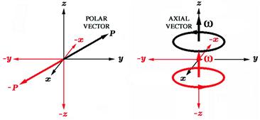
The triple scalar product, given by
 (12.33)
represents the volume of a parallelepiped formed by the three vectors A, B, and C, as shown in Figure 12.7. A ![]() determinant changes sign when two rows are interchanged but preserves its value under a cyclic permutation, so that
determinant changes sign when two rows are interchanged but preserves its value under a cyclic permutation, so that
![]() (12.34)
(12.34)
For three polar vectors, the triple scalar product changes sign upon inversion. Such a quantity is known as a pseudoscalar, in contrast to a scalar, which is invariant to inversion.

Figure 12.7 Triple scalar product as volume of parallelepiped: base area = BC sin![]() , altitude = A cos
, altitude = A cos![]() , volume = ABC sin
, volume = ABC sin![]() cos
cos![]() .
.
You might also encounter the triple vector product![]() , which is a vector quantity. This can be evaluated using the Levi-Civita representation (12.30). The i component of the triple product can be written
, which is a vector quantity. This can be evaluated using the Levi-Civita representation (12.30). The i component of the triple product can be written
![]() (12.35)
(12.35)
where we have introduced new dummy indices as needed. Focus on the sum over k of the product of the Levi-Civita symbols ![]() . For nonzero contributions, i and j must be different from k, and likewise for
. For nonzero contributions, i and j must be different from k, and likewise for ![]() and m. We must have either that
and m. We must have either that ![]() or
or ![]() . Therefore
. Therefore
![]() (12.36)
(12.36)
Since a sum containing a Kronecker delta reduces to a single term, we find
![]() (12.37)
(12.37)
Therefore, in full vector notation,
![]() (12.38)
(12.38)
which has the popular mnemonic “BAC(K) minus CAB.”
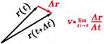
12.5 Vector Velocity and Acceleration
A particle moving in three dimensions can be represented by a time-dependent displacement vector:
![]() (12.39)
(12.39)
The velocity of the particle is the time derivative of ![]()
![]() (12.40)
(12.40)
as represented in Figure 12.8. The Cartesian components of velocity are
![]() (12.41)
(12.41)
The magnitude of the velocity vector is the speed:
![]() (12.42)
(12.42)
The velocity vector will be parallel to the displacement only if the particle is moving in a straight line. In Figure 12.8, ![]() can clearly be in a different direction. Thus, v(t) need not, in general, be parallel to r(t).
can clearly be in a different direction. Thus, v(t) need not, in general, be parallel to r(t).
Acceleration is the time derivative of velocity. We find
![]() (12.43)
(12.43)
with Cartesian components
![]() (12.44)
(12.44)
12.6 Circular Motion
Figure 12.9 represents a particle moving in a circle of radius r in the x, y-plane. Assuming a constant angular velocity of ![]() radians/s, the angular position of the particle is given by
radians/s, the angular position of the particle is given by ![]() . Cartesian coordinates can be defined with
. Cartesian coordinates can be defined with ![]() , so that
, so that
![]() (12.45)
(12.45)
Differentiation with respect to ![]() gives the velocity
gives the velocity
![]() (12.46)
(12.46)
As we have seen, the axial vector representing angular velocity is given by ![]() . Thus,
. Thus,
![]() (12.47)
(12.47)
and
![]() (12.48)
(12.48)
in agreement with Eq. (12.22).
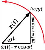
Figure 12.9 Displacement vector r(t) for particle moving in a circular path with angular velocity ![]() . The x- and y-components of r are shown.
. The x- and y-components of r are shown.
To find the acceleration of a particle in uniform circular motion, note that ![]() is a time-independent vector, so that
is a time-independent vector, so that
![]() (12.49)
(12.49)
In this case acceleration represents a change in the direction of the velocity vector, while the magnitude v remains constant. Using the right-hand rule, the acceleration is seen to be directed toward the center of the circle. This is known as centripetal acceleration, centripetal meaning “center seeking.” The magnitude of the centripetal acceleration is
![]() (12.50)
(12.50)
The force which causes centripetal acceleration is called centripetal force. By Newton’s second law
![]() (12.51)
(12.51)
For example, gravitational attraction to the Sun provides the centripetal force which keeps planets in nearly elliptical orbits. The effect known as centrifugal force is actually an artifice. It actually represents the tendency of a body to continue moving in a straight line, according to Newton’s first law. It might be naı¨vely perceived as a force away from the center. Actually, it is the centripetal force which keeps a body moving along a curved path, in resistance to this inertial tendency.
12.7 Angular Momentum
The linear momentum![]() is a measure of inertia for a particle moving in a straight line. Accordingly, Newton’s second law can be elegantly written
is a measure of inertia for a particle moving in a straight line. Accordingly, Newton’s second law can be elegantly written
![]() (12.52)
(12.52)
A result applying to angular motion can be obtained by taking the vector product of Newton’s law:
![]() (12.53)
(12.53)
The last equality follows from
![]() (12.54)
(12.54)
and the fact that ![]() . Angular momentum—more precisely, orbital angular momentum—is defined by
. Angular momentum—more precisely, orbital angular momentum—is defined by
![]() (12.55)
(12.55)
The analog of Eq. (12.52) for angular motion is
![]() (12.56)
(12.56)
where ![]() is called the torque or turning force. The law of conservation of angular momentum implies that, in the absence of external torque, a system will continue in its rotational motion.
is called the torque or turning force. The law of conservation of angular momentum implies that, in the absence of external torque, a system will continue in its rotational motion.
Consider a particle of mass m in angular motion with the angular velocity vector ![]() . The angular momentum can be related to the angular velocity using Eqs. (12.48) and (12.38):
. The angular momentum can be related to the angular velocity using Eqs. (12.48) and (12.38):
![]() (12.57)
(12.57)
where ![]() is the moment of inertia tensor, represented by the
is the moment of inertia tensor, represented by the ![]() matrix
matrix
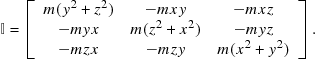 (12.58)
Tensors are the next member of the hierarchy which begins with scalars and vectors. The dot product of a tensor with a vector gives another vector. Usually the moment of inertia is defined for a rigid body, a system of particles with fixed relative coordinates. We must then replace ![]() in the matrix by the corresponding summation over all particles,
in the matrix by the corresponding summation over all particles, ![]() , and so forth. We will focus on the simple case of circular motion, with r being perpendicular to
, and so forth. We will focus on the simple case of circular motion, with r being perpendicular to ![]() as in Figure 12.9. This implies that
as in Figure 12.9. This implies that ![]() , so that the moment of inertia reduces to a scalar:
, so that the moment of inertia reduces to a scalar:
![]() (12.59)
(12.59)
Moment of inertia is a measure of a system’s resistance to change in its rotational motion, in the same way that mass is a measure of resistance to change in linear motion.
The kinetic energy for a mass in circular motion can be expressed in terms of the angular frequency. We find
![]() (12.60)
(12.60)
This can also be expressed
![]() (12.61)
(12.61)
Evidently, relations for linear motion can be transformed to their analogs for angular motion with the substitutions: ![]() . Here is a handy table giving the linear and angular equivalents for some mechanical variables:
. Here is a handy table giving the linear and angular equivalents for some mechanical variables:

12.8 Gradient of a Scalar Field
A scalar field ![]() can be represented graphically by a family of surfaces on which the field has a sequence of constant values (see Figure 12.10). If the scalar quantity is temperature, the surfaces are called isotherms. Analogously, barometric pressure is represented by isobars and electrical potential by equipotentials. (The less-familiar generic term for constant-value surfaces of a scalar field is isopleths.) When the position vector
can be represented graphically by a family of surfaces on which the field has a sequence of constant values (see Figure 12.10). If the scalar quantity is temperature, the surfaces are called isotherms. Analogously, barometric pressure is represented by isobars and electrical potential by equipotentials. (The less-familiar generic term for constant-value surfaces of a scalar field is isopleths.) When the position vector ![]() is changed by an infinitesimal
is changed by an infinitesimal ![]() , the change in
, the change in ![]() is given by the total differential [see Eq. (11.12)]
is given by the total differential [see Eq. (11.12)]
![]() (12.62)
(12.62)
This has the form of a scalar product of the differential displacement ![]() with the gradient vector
with the gradient vector
![]() (12.63)
(12.63)
In particular
![]() (12.64)
(12.64)
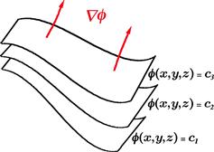
Figure 12.10 Gradients ![]() of a scalar field shown as red arrows. The gradient at every point
of a scalar field shown as red arrows. The gradient at every point ![]() is normal to the surface of constant
is normal to the surface of constant ![]() in the direction of maximum increase of
in the direction of maximum increase of ![]() .
.
When ![]() happens to lie within one of the surfaces of constant
happens to lie within one of the surfaces of constant ![]() , then
, then ![]() , which implies that the gradient
, which implies that the gradient ![]() at every point is normal to the surface
at every point is normal to the surface ![]() containing that point. This is shown in Figure 12.10, with arrows representing gradient vectors. Where constant
containing that point. This is shown in Figure 12.10, with arrows representing gradient vectors. Where constant ![]() surfaces are closer together, the function must be changing rapidly and the magnitude of
surfaces are closer together, the function must be changing rapidly and the magnitude of ![]() is correspondingly larger. This is more easily seen in a two-dimensional contour map, Figure 12.11. The gradient at
is correspondingly larger. This is more easily seen in a two-dimensional contour map, Figure 12.11. The gradient at ![]() points in the direction of maximum increase of
points in the direction of maximum increase of ![]() . The symbol
. The symbol ![]() is called “del” or “nabla” and stands for the vector differential operator
is called “del” or “nabla” and stands for the vector differential operator
![]() (12.65)
(12.65)
Sometimes ![]() is written
is written ![]() .
.
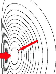
Figure 12.11 Two-dimensional contour map showing, for example, the elevation around a hill. Where the contours are more closely spaced, the terrain is steeper and the gradient larger in magnitude. This is indicated by the thicker arrow.
The change in a scalar field ![]() along a unit vector
along a unit vector ![]() is called the directional derivative, defined by
is called the directional derivative, defined by
![]() (12.66)
(12.66)
A finite change in the scalar field ![]() as r moves from
as r moves from ![]() to
to ![]() over a path C is given by the line integral
over a path C is given by the line integral
![]() (12.67)
(12.67)
Work in mechanics is given by a line integral over force: ![]() . The work done by the system is the negative of this quantity. Thus, for a conservative system, force is given by the negative gradient of potential energy:
. The work done by the system is the negative of this quantity. Thus, for a conservative system, force is given by the negative gradient of potential energy: ![]() . An analogous relation holds in electrostatics between the electric field and the potential:
. An analogous relation holds in electrostatics between the electric field and the potential: ![]() .
.
Problem 12.8.1
The force between two electrical charges ![]() and
and ![]() separated by a displacement vector r (in three dimensions) is given by Coulomb’s law,
separated by a displacement vector r (in three dimensions) is given by Coulomb’s law, ![]() . Derive the potential-energy function
. Derive the potential-energy function ![]() .
.
12.9 Divergence of a Vector Field
One of the cornerstones of modern physics is the conservation of electric charge. If an element of volume contains a certain quantity of charge, that quantity can change only when charge flows through the boundary of the volume. The charge per unit volume measured in Coulombs per unit volume (C/m3), is designated the charge density![]() . The flow of charge across unit area per unit time is represented by the current densityJ(r, t). The current density at a point r equals the product of the density and the instantaneous velocity of charge at that point:
. The flow of charge across unit area per unit time is represented by the current densityJ(r, t). The current density at a point r equals the product of the density and the instantaneous velocity of charge at that point:
![]() (12.68)
(12.68)
This is dimensionally consistent since
![]() (12.69)
(12.69)
Note that J(r, t) and v(r, t) are vector fields, while ![]() is a scalar field.
is a scalar field.
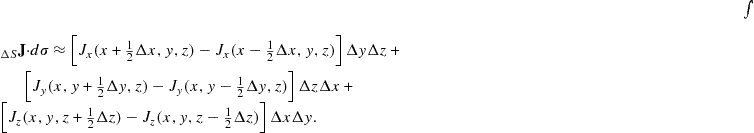
Consider the element of volume ![]() in Cartesian coordinates, shown in Figure 12.12. Designating the coordinates at the center by
in Cartesian coordinates, shown in Figure 12.12. Designating the coordinates at the center by ![]() , the middle of the faces normal to the x-direction are
, the middle of the faces normal to the x-direction are ![]() and
and ![]() , and analogously for the faces normal to the other two directions. The electric charge contained in
, and analogously for the faces normal to the other two directions. The electric charge contained in ![]() can be approximated by
can be approximated by ![]() . The net charge leaving
. The net charge leaving ![]() per unit time is then equal to the integral over the current density normal to the surface
per unit time is then equal to the integral over the current density normal to the surface ![]() enclosing the element of volume. Such a surface integral can be written
enclosing the element of volume. Such a surface integral can be written ![]() , where
, where ![]() , an element of area with the direction of the outward normal from the surface. In the present case, the surface integral is the sum of contributions from the six faces of
, an element of area with the direction of the outward normal from the surface. In the present case, the surface integral is the sum of contributions from the six faces of ![]() , thus
, thus
 (12.70)
Divide each side by ![]() and let the element of volume be shrunken to a point. In the limit
and let the element of volume be shrunken to a point. In the limit ![]() , the terms containing
, the terms containing ![]() reduce to a partial derivative, as follows:
reduce to a partial derivative, as follows:
![]() (12.71)
(12.71)
Adding the analogous ![]() and
and ![]() contributions, we find
contributions, we find
![]() (12.72)
(12.72)
The right-hand side has the structure of a scalar product of ![]() with
with ![]() :
:
![]() (12.73)
(12.73)
called the divergence of J (also written div J).
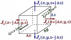
Figure 12.12 Flux of a vector field J out of an element of volume ![]() with surface
with surface ![]() , for derivation of the divergence theorem.
, for derivation of the divergence theorem.
The divergence of the current density at a point x,y,z represents the net outward flux of electric charge from that point. Since electric charge is conserved, the flow of charge from every point must be balanced by a reduction of the charge density ![]() in the vicinity of that point. This leads to the equation of continuity
in the vicinity of that point. This leads to the equation of continuity
![]() (12.74)
(12.74)
In the steady-state case, in which there is no accumulation of charge at any point, the equation of continuity reduces to
![]() (12.75)
(12.75)
In defining the divergence of a vector field A(r, t), we have transformed an integration over surface area into an integration over volume, as shown in Figure 12.12. When two such elements of volume are adjacent, the contribution from their interface cancels out, since flux into one element is exactly canceled by flux out of the adjacent element. By adding together an infinite number of infinitesimal elements, the result can be generalized to a finite volume of arbitrary shape. We arrive thereby at the divergence theorem (also known as Gauss’ theorem):
![]() (12.76)
(12.76)
A differential element of volume is conventionally written ![]() . Sometimes the notation
. Sometimes the notation ![]() is used for S, to indicate the surface area enclosing the volume V.
is used for S, to indicate the surface area enclosing the volume V.
The divergence of the gradient of a scalar field occurs in several fundamental equations of electromagnetism, wave theory, and quantum mechanics. In Cartesian coordinates
![]() (12.77)
(12.77)
The operator
![]() (12.78)
(12.78)
is called the Laplacian or “del squared.” Sometimes ![]() is abbreviated as
is abbreviated as ![]() .
.
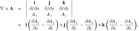
12.10 Curl of a Vector Field
As we have seen, a vector field can be imagined as some type of flow. We used this idea in defining the divergence. Another aspect of flow might be circulation, in the sense of a local angular velocity. Figure 12.13 gives a schematic pictorial representation of vector fields with outward flux (left) and with circulation (right). To be specific, consider a rectangular element in the x, y-plane as shown in Figure 12.14. The center of the rectangle at (x, y), the four sides are at ![]() and
and ![]() . The area if the rectangle is
. The area if the rectangle is ![]() . The circulation of a vector field A(r) around the rectangle in the counterclockwise sense is approximated by
. The circulation of a vector field A(r) around the rectangle in the counterclockwise sense is approximated by
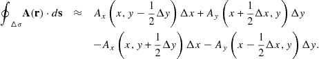 (12.79)
Next we divide both sides by ![]() and take the limits
and take the limits ![]() . Since
. Since
 (12.80)
and
![]() (12.81)
(12.81)
we find
![]() (12.82)
(12.82)
It can be recognized that the difference of partial derivatives represents the z-component of a cross product involving the vector operator ![]() :
:
 (12.83)
The vector field ![]() is called the curl of
is called the curl of![]() , also written curl A. For an element of area in an arbitrary orientation, we find the limit
, also written curl A. For an element of area in an arbitrary orientation, we find the limit
![]() (12.84)
(12.84)
where ![]() is directed normal to the element of area. An arbitrary surface, such as the one drawn in Figure 12.15, can be formed from an infinite number of infinitesimal elements of area such as Figure 12.14. The line integral of a vector field A(r) counterclockwise around a path closed C can be related to surface integral of
is directed normal to the element of area. An arbitrary surface, such as the one drawn in Figure 12.15, can be formed from an infinite number of infinitesimal elements of area such as Figure 12.14. The line integral of a vector field A(r) counterclockwise around a path closed C can be related to surface integral of ![]() over the enclosed area by Stokes’ theorem:
over the enclosed area by Stokes’ theorem:
![]() (12.85)
(12.85)
In two dimensions, Stokes’ theorem reduces to Green’s theorem (11.75):
![]() (12.86)
(12.86)
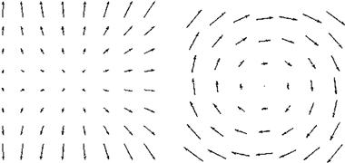
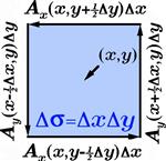
Figure 12.14 Circulation of a vector field A(r) about an element of area ![]() . In the limit
. In the limit ![]() , this gives the z-component of the curl
, this gives the z-component of the curl ![]() .
.
For arbitrary scalar and vector fields ![]() and
and ![]() the following identities involving divergence and curl can be readily derived:
the following identities involving divergence and curl can be readily derived:
![]() (12.87)
(12.87)
and
![]() (12.88)
(12.88)
An intriguing combination is ![]() also known as “curl curl” (Curl Curl Beach is a suburban resort outside Sydney, Australia). This has the form of a triple vector product (12.38). We must be careful about the order of factors, however, since
also known as “curl curl” (Curl Curl Beach is a suburban resort outside Sydney, Australia). This has the form of a triple vector product (12.38). We must be careful about the order of factors, however, since ![]() is a differential operator. If the vector
is a differential operator. If the vector ![]() is always kept on the right of the
is always kept on the right of the ![]() ’s, we obtain the correct result:
’s, we obtain the correct result:
![]() (12.89)
(12.89)
Note that ![]() is a vector quantity such that
is a vector quantity such that
![]() (12.90)
(12.90)
12.11 Maxwell’s Equations
These four fundamental equations of electromagnetic theory can be very elegantly expressed in terms of the vector operators, divergence and curl. The first Maxwell equation is a generalization of Coulomb’s law for the electric field of a point charge:
![]() (12.91)
(12.91)
where Q is the electric charge and ![]() , the permittivity of free space. The unit vector
, the permittivity of free space. The unit vector ![]() indicates that the field is directed radially outward from the charge (or radially inward for a negative charge). We write
indicates that the field is directed radially outward from the charge (or radially inward for a negative charge). We write
![]() (12.92)
(12.92)
Since ![]() represents an element of area with an outward-directed normal, this can be transformed into the integral relationship
represents an element of area with an outward-directed normal, this can be transformed into the integral relationship
![]() (12.93)
(12.93)
where ![]() is the charge density within a sphere of volume V with surface area S. But by the divergence theorem,
is the charge density within a sphere of volume V with surface area S. But by the divergence theorem,
![]() (12.94)
(12.94)
The corresponding differential form is then the first of Maxwell’s equations:
![]() (12.95)
(12.95)
Free magnetic poles, the magnetic analog of electric charges, have never been observed (although their existence has been postulated in some theories). This implies that the divergence of the magnetic induction B equals zero, which serves as the second Maxwell equation:
![]() (12.96)
(12.96)
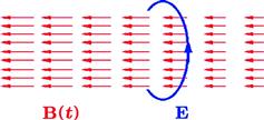
According to Faraday’s law of electromagnetic induction, a time-varying magnetic field induces an electromotive force in a conducting loop through which the magnetic field threads, as shown in Figure 12.16. This is somewhat suggestive of a linear relationship between the time derivative of the magnetic induction and the curl of the electric field. Indeed, the appropriate equation is
![]() (12.97)
(12.97)
Oersted discovered that an electric current produces a magnetic field winding around it, as shown in Figure 12.17. The quantitative result, suggested by analogy with Eq. (12.97), is Ampère’s law:
![]() (12.98)
(12.98)
where ![]() is the permeability of free space. Maxwell showed that Ampère’s law must be incomplete by the following argument. Taking the divergence of (12.98) we find
is the permeability of free space. Maxwell showed that Ampère’s law must be incomplete by the following argument. Taking the divergence of (12.98) we find
![]() (12.99)
(12.99)
since the divergence of a curl is identically zero [Eq. (12.88)]. This is consistent only for the special case of steady currents [Eq. (12.75)]. To make the right-hand side accord with the full equation of continuity, Eq. (12.74), we can write
![]() (12.100)
(12.100)
This is still equivalent to 0 = 0 but suggests by (12.95) that
![]() (12.101)
(12.101)
With Maxwell’s displacement current hypothesis, the generalization of Ampère’s law is
![]() (12.102)
(12.102)
the added term being known as the displacement current.

We have given the forms of Maxwell’s equations in free space. In material media, two auxilliary fields are defined: the electric displacement ![]() and the magnetic field
and the magnetic field ![]() . In terms of these, we can write compact forms for Maxwell’s equations in SI units:
. In terms of these, we can write compact forms for Maxwell’s equations in SI units:
![]() (12.103)
(12.103)
In the absence of charges and currents (![]() and
and ![]() ), Maxwell’s equations reduce to
), Maxwell’s equations reduce to
![]() (12.104)
(12.104)
Taking the curl of the third equation, the time derivative of the fourth and eliminating the terms in B, we find
![]() (12.105)
(12.105)
Using the curl curl equation (12.89) and noting that ![]() we obtain the wave equation for the electric field:
we obtain the wave equation for the electric field:
![]() (12.106)
(12.106)
An analogous derivation shows that the magnetic induction also satisfies the wave equation:
![]() (12.107)
(12.107)
Maxwell proposed that Eqs. (12.106) and (12.107) describe the propagation of electromagnetic waves at the speed of light
![]() (12.108)
(12.108)
Note that this conclusion would not have been possible without the displacement current hypothesis.
By virtue of the vector identities (12.87) and (12.88), the two vector fields E and B can be represented by electromagnetic potentials—one vector field and one scalar field. The second Maxwell equation (12.96) suggests that the magnetic induction can be written
![]() (12.109)
(12.109)
where A(r, t) is called the vector potential. Substituting this into the third Maxwell equation (12.97), we can write
![]() (12.110)
(12.110)
This suggests that the quantity in parentheses can be represented as the divergence of a scalar function, conventionally written in the form
![]() (12.111)
(12.111)
where ![]() is called the scalar potential. In the time-independent case, the latter reduces to the Coulomb or electrostatic potential, with
is called the scalar potential. In the time-independent case, the latter reduces to the Coulomb or electrostatic potential, with ![]() . The electric field and magnetic induction are uniquely determined by the scalar and vector potentials:
. The electric field and magnetic induction are uniquely determined by the scalar and vector potentials:
![]() (12.112)
(12.112)
The converse is not true, however. Consider the alternative choice of electromagnetic potentials
![]() (12.113)
(12.113)
where ![]() is an arbitrary function. The modified potentials
is an arbitrary function. The modified potentials ![]() and
and ![]() can be verified to give the sameE and B as the original potentials. This property of electromagnetic fields is called gauge invariance. Extension of this principle to quantum theory leads to the concept of gauge fields, which provides the framework of the standard model for elementary particles and their interactions.
can be verified to give the sameE and B as the original potentials. This property of electromagnetic fields is called gauge invariance. Extension of this principle to quantum theory leads to the concept of gauge fields, which provides the framework of the standard model for elementary particles and their interactions.
12.12 Covariant Electrodynamics
Electromagnetic theory can be very compactly expressed in Minkowski four-vector notation. Historically, it was this symmetry of Maxwell’s equations which led to the Special Theory of Relativity. Now that we know about partial derivatives, the gradient four-vector can be defined. This is a covariant operator
![]() (12.114)
(12.114)
The corresponding contravariant operator is
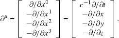 (12.115)
The scalar product gives
![]() (12.116)
(12.116)
The D’Alembertian operator![]() is defined by
is defined by
![]() (12.117)
(12.117)
a notation is suggested by analogy with the symbol ![]() for the Laplacian operator
for the Laplacian operator ![]() . The wave equations (12.106) and (12.107) can thus be compactly written
. The wave equations (12.106) and (12.107) can thus be compactly written
![]() (12.118)
(12.118)
For the Minkowski signature ![]() ,
, ![]() . The alternative choice of signature
. The alternative choice of signature ![]() implies
implies ![]() . To confuse matters further,
. To confuse matters further, ![]() is sometimes written in place of
is sometimes written in place of ![]() .
.
The equation of continuity for electric charge (12.74) has the structure of a four-dimensional divergence
![]() (12.119)
(12.119)
in terms of the charge-current four-vector
 (12.120)
In Lorenz gauge, the function ![]() in Eqs. (12.113) is chosen such that
in Eqs. (12.113) is chosen such that ![]() . The scalar and vector potentials are then related by the Lorenz condition
. The scalar and vector potentials are then related by the Lorenz condition
![]() (12.121)
(12.121)
This can also be expressed as a four-dimensional divergence
![]() (12.122)
(12.122)
in terms of a four-vector potential
 (12.123)
Maxwell’s equations in Lorenz gauge can be expressed by a single Minkowski-space equation
![]() (12.124)
(12.124)
where the ![]() component gives
component gives
![]() (12.125)
(12.125)
(Incidentally, the Lorenz gauge was proposed by the Danish physicist Ludvig Lorenz. It is often erroneously designated “Lorentz gauge,” after the more famous Dutch physicist Hendrik Lorentz. In fact, the condition does fulfill the property known as Lorentz invariance.)
The electric and magnetic fields obtained from the potentials using (12.112) can be represented by a single relation for the electromagnetic field tensor
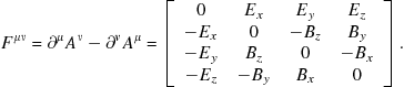 (12.126)
Maxwell’s equations, in terms of the electromagnetic field tensor, can be written:
![]() (12.127)
(12.127)
Problem 12.12.1
An electromagnetic field dual tensor can be defined by
![]()
where ![]() is the four-dimensional Levi-Civita tensor. Verify that
is the four-dimensional Levi-Civita tensor. Verify that

This can be obtained from the ![]() tensor by the formal substitutions
tensor by the formal substitutions ![]() and
and ![]() .
.
Problem 12.12.2
Show that the second of Maxwell’s equations in (12.127) can be written more compactly as
![]()
12.13 Curvilinear Coordinates
Vector equations can provide an elegant abstract formulation of physical laws, but, in order to solve problems, it is usually necessary to express these equations in a particular coordinate system. Thus far we have considered Cartesian coordinates almost exclusively. Another choice, for example, cylindrical or spherical coordinates, might prove more appropriate, depending on the symmetry of the problem.
We will consider the general class of orthogonal curvilinear coordinates, designated ![]() , whose coordinate surfaces always mutually intersect at right angles. The Cartesian coordinates of a point in three-dimensional space can be expressed in terms of a set of curvilinear coordinates by relations of the form
, whose coordinate surfaces always mutually intersect at right angles. The Cartesian coordinates of a point in three-dimensional space can be expressed in terms of a set of curvilinear coordinates by relations of the form
![]() (12.128)
(12.128)
The differentials of the Cartesian coordinates are
![]() (12.129)
(12.129)
with analogous expressions for dy and dz. Thus a differential element of displacement ![]() can be written
can be written
![]() (12.130)
(12.130)
where ![]() are unit vectors with respect to the curvilinear coordinates
are unit vectors with respect to the curvilinear coordinates ![]() and
and ![]() are scale factors. As shown in Figure 12.18, the elements of length in the three coordinate directions are equal to
are scale factors. As shown in Figure 12.18, the elements of length in the three coordinate directions are equal to ![]() ,
, ![]() , and
, and ![]() . The element of volume is evidently given by
. The element of volume is evidently given by
![]() (12.131)
(12.131)
where the ![]() are, in general, functions of
are, in general, functions of ![]() .
.
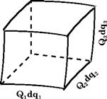
We can evidently identify
![]() (12.132)
(12.132)
so that the element of volume can be equated to a triple scalar product (cf Section 12.4):
 (12.133)
This can therefore be connected to the Jacobian determinant:
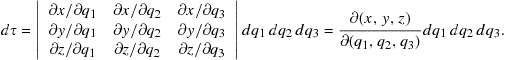 (12.134)
The components of the gradient vector represent directional derivatives of a function. For example, the change in the function ![]() along the
along the ![]() -direction is given by the ratio of
-direction is given by the ratio of ![]() to the element of length
to the element of length ![]() . Thus, the gradient in curvilinear coordinates can be written
. Thus, the gradient in curvilinear coordinates can be written
![]() (12.135)
(12.135)
The divergence ![]() represents the limiting value of the net outward flux of the vector quantity
represents the limiting value of the net outward flux of the vector quantity ![]() per unit volume. Referring to Figure 12.19, the net flux of the component
per unit volume. Referring to Figure 12.19, the net flux of the component ![]() in the
in the ![]() -direction is given by the difference between the outward contributions
-direction is given by the difference between the outward contributions ![]() on the two shaded faces. As the volume element approaches a point, this reduces to
on the two shaded faces. As the volume element approaches a point, this reduces to
![]() (12.136)
(12.136)
Adding the analogous contributions from the ![]() - and
- and ![]() -directions and diving by the volume
-directions and diving by the volume ![]() , we obtain the general result for the divergence in curvilinear coordinates:
, we obtain the general result for the divergence in curvilinear coordinates:
![]() (12.137)
(12.137)
The curl in curvilinear coordinates is given by
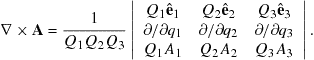 (12.138)
The Laplacian is the divergence of the gradient, so that substitution of (12.135) into (12.137) gives
![]() (12.139)
(12.139)

The three most common coordinate systems in physical applications are Cartesian, with ![]() , cylindrical, with
, cylindrical, with ![]() , and spherical polar, with
, and spherical polar, with ![]() . We frequently encounter the spherical polar volume element
. We frequently encounter the spherical polar volume element
![]() (12.140)
(12.140)
and the Laplacian operator
![]() (12.141)
(12.141)
Problem 12.13.1
Determine the forms of the scalar and vector products, ![]() and
and ![]() , in terms of the components of
, in terms of the components of ![]() and
and ![]() in spherical polar coordinates.
in spherical polar coordinates.