Algebra
3.1 Symbolic Variables
Algebra is a lot like arithmetic but deals with symbolic variables in addition to numbers. Very often these include ![]() , and/or z, especially for “unknown” quantities which is often your job to solve for. Earlier letters of the alphabet such as
, and/or z, especially for “unknown” quantities which is often your job to solve for. Earlier letters of the alphabet such as ![]() are often used for “constants,” quantities whose values are determined by assumed conditions before you solve a particular problem. Most English letters find use somewhere as either variables or constants. Remember that variables are case sensitive, so X designates a different quantity than x. As the number of mathematical symbols in a technical subject proliferates, the English (really Latin) alphabet becomes inadequate to name all the needed variables. So Greek letters have to be used in addition. Here are the 24 letters of the Greek alphabet:
are often used for “constants,” quantities whose values are determined by assumed conditions before you solve a particular problem. Most English letters find use somewhere as either variables or constants. Remember that variables are case sensitive, so X designates a different quantity than x. As the number of mathematical symbols in a technical subject proliferates, the English (really Latin) alphabet becomes inadequate to name all the needed variables. So Greek letters have to be used in addition. Here are the 24 letters of the Greek alphabet:

If you ever pledged a fraternity or sorority, they probably made you memorize these Greek letters (but your advantage was probably nullified by too much partying). Several upper-case Greek letters are identical to English ones, and so provide nothing new. The most famous Greek symbol is ![]() , which stands for the universal ratio between the circumference and diameter of a circle:
, which stands for the universal ratio between the circumference and diameter of a circle: ![]()
The fundamental entity in algebra is an equation, consisting of two quantities connected by an equal sign. An equation can be thought of as a two pans of a scale, like the one held up by blindfolded Ms. Justice (Figure 3.1). When the weights of the two pans are equal, the scale is balanced. Weights can be added, subtracted, multiplied, or interchanged in such a way that the balance is maintained. Each such move has its analog as a legitimate algebraic operation which maintains the equality. The purpose of such operations is to get the equation into some desired form or to “solve” for one of its variables, which means to isolate it, usually on the left-hand side of the equation. Einstein commented on algebra, “It’s a merry science. When the animal we are hunting cannot be caught, we call it x temporarily and continue to hunt until it is bagged.”

3.2 Legal and Illegal Algebraic Manipulations
Let’s start with a simple equation
![]() (3.1)
(3.1)
Following are the results of some legal things you can do
![]() (3.2)
(3.2)
![]() (3.3)
(3.3)
![]() (3.4)
(3.4)
![]() (3.5)
(3.5)
![]() (3.6)
(3.6)
![]() (3.7)
(3.7)
Here is a very tempting but ILLEGAL manipulation:
![]() (3.8)
(3.8)
A very useful reduction for ratios makes use of crossmultiplication:
![]() (3.9)
(3.9)
Note that you can validly go in either direction.
For the addition and multiplication of fractions, the two key relationships are:
![]() (3.10)
(3.10)
The distributive law for multiplication states that
![]() (3.11)
(3.11)
This implies
![]() (3.12)
(3.12)
In particular
![]() (3.13)
(3.13)
Another useful relationship comes from
![]() (3.14)
(3.14)
These last two formulas are worth having in your readily available memory.
Complicated algebraic expressions are best handled nowadays using symbolic math programs such as MathematicaTM.
Cancellation is a wonderful way to simplify formulas. Consider
![]() (3.15)
(3.15)
where the symbols in gray boxes are to be crossed out. But don’t spoil everything by trying to cancel the bs or cs as well. The analogous cancellation can be done on the two sides of an equation:
![]() (3.16)
(3.16)
For your amusement, here is a “proof” that ![]() . The following sequence of algebraic operations is entirely legitimate, except for one little item of trickery snuck in. Suppose we are given that
. The following sequence of algebraic operations is entirely legitimate, except for one little item of trickery snuck in. Suppose we are given that
![]() (3.17)
(3.17)
Then
![]() (3.18)
(3.18)
and
![]() (3.19)
(3.19)
Factoring both sides of the equation,
![]() (3.20)
(3.20)
We can then simplify by cancellation of ![]() to get
to get
![]() (3.21)
(3.21)
But since ![]() this means that 2 = 1! Where did we go wrong?
this means that 2 = 1! Where did we go wrong?
Once you recover from shock, note that ![]() . And division by 0 is not legitimate. It is, in fact, true that
. And division by 0 is not legitimate. It is, in fact, true that ![]() , but we can’t cancel out the zeros!
, but we can’t cancel out the zeros!
3.3 Factor-Label Method
A very useful technique for converting physical quantities to alternative sets of units is the factor-label method. The units themselves are regarded as algebraic quantities subject to the rules of arithmetic, particularly to cancellation. To illustrate, let us calculate the speed of light in miles/s, given the metric value ![]() . First write this as an equation
. First write this as an equation
![]() (3.22)
(3.22)
Now ![]() , which we can express in the form of a simple equation
, which we can express in the form of a simple equation
![]() (3.23)
(3.23)
Multiplying Eq. (3.22) by 1 in the form of the last expression, and cancelling the units m from numerator and denominator, we find
![]() (3.24)
(3.24)
We continue by multiplying the result by successive factors of 1, expressed in appropriate forms, namely
![]() (3.25)
(3.25)
Thus we can continue our multiplication and cancellation sequence beginning with (3.24):
![]() (3.26)
(3.26)
a number well known to readers of science fiction. Note that singular and plural forms, e.g. “foot” and “feet,” are regarded as equivalent for purposes of cancellation.
As another example, let us calculate the number of seconds in a year. Proceeding as before:
![]() (3.27)
(3.27)
To within about 0.5%, we can approximate
![]() (3.28)
(3.28)
3.4 Powers and Roots
You remember of course that ![]() and
and ![]() , so
, so ![]() . It is also easy to see that
. It is also easy to see that ![]() . The general formulas are:
. The general formulas are:
![]() (3.29)
(3.29)
and
![]() (3.30)
(3.30)
For the case ![]() with
with ![]() , the last result implies the frequently encountered identity
, the last result implies the frequently encountered identity
![]() (3.31)
(3.31)
From (3.29) with ![]()
![]() (3.32)
(3.32)
(not ![]() ). More generally,
). More generally,
![]() (3.33)
(3.33)
Note that ![]() , an instance of the general result
, an instance of the general result
![]() (3.34)
(3.34)
You should be familiar with the limits as ![]()
![]() (3.35)
(3.35)
and
![]() (3.36)
(3.36)
Remember that ![]() while
while ![]() . Dividing by zero sends some calculators and computers into a tizzy.
. Dividing by zero sends some calculators and computers into a tizzy.
Consider a more complicated expression, say a ratio of polynomials
![]()
In the limit as ![]() ,
, ![]() becomes negligible compared to
becomes negligible compared to ![]() , as does any constant term. Therefore
, as does any constant term. Therefore
![]() (3.37)
(3.37)
In the limit as ![]() , on the other hand, all positive powers of x eventually become negligible compared to a constant. And so
, on the other hand, all positive powers of x eventually become negligible compared to a constant. And so
![]() (3.38)
(3.38)
Using (3.32) with ![]() we find
we find
![]() (3.39)
(3.39)
Therefore ![]() must mean the square root of x:
must mean the square root of x:
![]() (3.40)
(3.40)
More generally
![]() (3.41)
(3.41)
and evidently
![]() (3.42)
(3.42)
This also implies the equivalence
![]() (3.43)
(3.43)
Finally, consider the product ![]() . The general rule is
. The general rule is
![]() (3.44)
(3.44)
3.5 Logarithms
Inverse operationsare pairs of mathematical manipulations in which one operation undoes the action of the other—for example, addition and subtraction, multiplication and division. The inverse of a number usually means its reciprocal, i.e. ![]() . The product of a number and its inverse (reciprocal) equals 1. Raising to a power and extraction of a root are evidently another pair of inverse operations. An alternative inverse operation for raising to a power is taking the logarithm. The following relations are equivalent:
. The product of a number and its inverse (reciprocal) equals 1. Raising to a power and extraction of a root are evidently another pair of inverse operations. An alternative inverse operation for raising to a power is taking the logarithm. The following relations are equivalent:
![]() (3.45)
(3.45)
in which a is called the base of the logarithm.
All the formulas for manipulating logarithms can be obtained from corresponding relations involving raising to powers. If ![]() then
then ![]() . The last relation is equivalent to
. The last relation is equivalent to ![]() , therefore
, therefore
![]() (3.46)
(3.46)
where base a is understood. If ![]() and
and ![]() , then
, then ![]() and
and ![]() . Therefore
. Therefore
![]() (3.47)
(3.47)
More generally,
![]() (3.48)
(3.48)
There is no simple reduction for ![]() —don’t fall into the trap mentioned in the Preface! Since
—don’t fall into the trap mentioned in the Preface! Since ![]() ,
,
![]() (3.49)
(3.49)
The identity ![]() implies that, for any base,
implies that, for any base,
![]() (3.50)
(3.50)
The log of a number less than 1 has a negative value. For any base ![]() ,
, ![]() , so that
, so that
![]() (3.51)
(3.51)
To find the relationship between logarithms of different bases, suppose ![]() , so
, so ![]() . Now, taking logs to the base a,
. Now, taking logs to the base a,
![]() (3.52)
(3.52)
In a more symmetrical form
![]() (3.53)
(3.53)
The slide rule, shown in Figure 3.2, is based on the principle that multiplication of two numbers is equivalent to adding their logarithms. Slide rules, once a distinguishing feature of science and engineering students, have been completely supplanted by hand-held calculators.
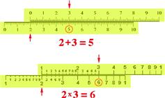
Figure 3.2 Principle of the slide rule. Top: Hypothetical slide rule for addition. To add 2 + 3, slide the 0 on the upper scale opposite 2 on the lower scale and look for 3 on the upper scale. The sum 5 appears below it. Bottom: Real slide rule based on logarithmic scale. To multiply ![]() , slide the 1 on the upper scale opposite 2 on the lower scale and look for 3 on the upper scale. The product 6 appears below it. Note that
, slide the 1 on the upper scale opposite 2 on the lower scale and look for 3 on the upper scale. The product 6 appears below it. Note that ![]() and that adding
and that adding ![]() gives
gives ![]() .
.
Logarithms to the base 10 are called Briggsian or common logarithms. Before the advent of scientific calculators, these were an invaluable aid to numerical computation. Section 1.3 on “Powers of 10” was actually a tour on the ![]() scale. Logarithmic scales give more convenient numerical values in many scientific applications. For example, in chemistry, the hydrogen ion concentration (technically, the activity) of a solution is represented by
scale. Logarithmic scales give more convenient numerical values in many scientific applications. For example, in chemistry, the hydrogen ion concentration (technically, the activity) of a solution is represented by
![]() (3.54)
(3.54)
A neutral solution has a pH of 7, corresponding to ![]() . An acidic solution has
. An acidic solution has ![]() while a basic solution has
while a basic solution has ![]() . Another well-known logarithmic measure is the Richter scale for earthquake magnitudes.
. Another well-known logarithmic measure is the Richter scale for earthquake magnitudes. ![]() is a minor tremor of some standard intensity as measured by a seismometer. The magnitude increases by 1 for every 10-fold increase in intensity.
is a minor tremor of some standard intensity as measured by a seismometer. The magnitude increases by 1 for every 10-fold increase in intensity. ![]() is considered a “major” earthquake, capable of causing extensive destruction and loss of life. The largest magnitude in recorded history was
is considered a “major” earthquake, capable of causing extensive destruction and loss of life. The largest magnitude in recorded history was ![]() , for the great 1960 earthquake in Chile.
, for the great 1960 earthquake in Chile.
Of more fundamental mathematical significance are logarithms to the base ![]() , known as natural logarithms. We will explain the significance of e a little later. In most scientific usage the natural logarithm is written as “ln”
, known as natural logarithms. We will explain the significance of e a little later. In most scientific usage the natural logarithm is written as “ln”
![]() (3.55)
(3.55)
But be forewarned that most literature in pure mathematics uses “![]() ” to mean natural logarithm. Using (3.52) with
” to mean natural logarithm. Using (3.52) with ![]() and
and ![]()
![]() (3.56)
(3.56)
Logarithms to the base 2 can be associated with the binary number system. The value of ![]() (also written lg 2) is equal to the number of bits contained in the magnitude x. For example,
(also written lg 2) is equal to the number of bits contained in the magnitude x. For example, ![]() .
.
3.6 The Quadratic Formula
The two roots of the quadratic equation
![]() (3.57)
(3.57)
are given by one of the most useful formulas in elementary algebra. We don’t generally spend much time deriving formulas, but in this one instance, the derivation is very instructive. Consider the following very simple polynomial which is very easily factored:
![]() (3.58)
(3.58)
Suppose we were given instead ![]() . We can’t factor this as readily but here is an alternative trick. Knowing how the polynomial (3.58) factors we can write
. We can’t factor this as readily but here is an alternative trick. Knowing how the polynomial (3.58) factors we can write
![]() (3.59)
(3.59)
This makes use of a strategem called “completing the square.” In the more general case, we can write
![]() (3.60)
(3.60)
This suggests how to solve the quadratic equation (3.57). First complete the square involving the first two terms:
![]() (3.61)
(3.61)
so that
![]() (3.62)
(3.62)
Taking the square root:
 (3.63)
then leads to the famous quadratic formula
![]() (3.64)
(3.64)
The quantity
![]() (3.65)
(3.65)
is known as the discriminant of the quadratic equation. If ![]() the equation has two distinct real roots. For example,
the equation has two distinct real roots. For example, ![]() , with
, with ![]() , has the two roots
, has the two roots ![]() and
and ![]() . If
. If ![]() , the equation has two equal real roots. For example,
, the equation has two equal real roots. For example, ![]() , with
, with ![]() has the double root
has the double root ![]() . If the discriminant
. If the discriminant ![]() , the quadratic formula contains the square root of a negative number. This leads us to imaginary and complex numbers. Before about 1800, most mathematicians would have told you that the quadratic equation with negative discriminant has no solutions. Associated with this point of view, the square root of a negative number has acquired the designation “imaginary.” The sum of a real number with an imaginary is called a complex number. If we boldly accept imaginary and complex numbers, we are led to the elegant result that every quadratic equation has exactly two roots, whatever the sign of its discriminant. More generally, every nth-degree polynomial equation
, the quadratic formula contains the square root of a negative number. This leads us to imaginary and complex numbers. Before about 1800, most mathematicians would have told you that the quadratic equation with negative discriminant has no solutions. Associated with this point of view, the square root of a negative number has acquired the designation “imaginary.” The sum of a real number with an imaginary is called a complex number. If we boldly accept imaginary and complex numbers, we are led to the elegant result that every quadratic equation has exactly two roots, whatever the sign of its discriminant. More generally, every nth-degree polynomial equation
![]() (3.66)
(3.66)
has exactly n roots.
The simplest quadratic equation with imaginary roots is
![]() (3.67)
(3.67)
Applying the quadratic formula (3.64), we obtain the two roots
![]() (3.68)
(3.68)
As another example,
![]() (3.69)
(3.69)
has the roots
![]() (3.70)
(3.70)
Observe that whenever ![]() , the roots occur as conjugate pairs, one root containing
, the roots occur as conjugate pairs, one root containing ![]() and the other,
and the other, ![]() .
.
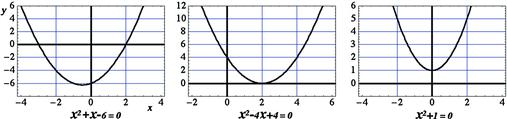
The three quadratic equations considered above can be solved graphically, as shown in Figure 3.3. The two points where the parabola representing the equation crosses the x-axis correspond to the real roots. For a double root, the curve is tangent to the x-axis. If there are no real roots, as in the case of ![]() , the curve does not intersect the x-axis.
, the curve does not intersect the x-axis.
Problem 3.6.1
Solve the quadratic equation ![]() .
.
3.7 Imagining i
If we an nth-degree polynomial does indeed have a total of n roots, then we must accept roots containing square roots of negative numbers—imaginary and complex numbers. The designation “imaginary” is an unfortunate accident of history since we will show that ![]() is, in fact, no more fictitious than 1 or 0—it’s just a different kind of number, with as much fundamental significance as those we respectfully call real numbers.
is, in fact, no more fictitious than 1 or 0—it’s just a different kind of number, with as much fundamental significance as those we respectfully call real numbers.
The square root of a negative number is a multiple of ![]() . For example,
. For example, ![]() . The imaginary unit is defined by
. The imaginary unit is defined by
![]() (3.71)
(3.71)
Consequently
![]() (3.72)
(3.72)
Clearly, there is no place on the axis of real numbers running from ![]() to
to ![]() to accommodate imaginary numbers. We are therefore forced to move into a higher dimension, representing all possible polynomial roots on a two-dimensional plane. This is known as a complex plane or Argand diagram, shown in Figure 3.4. The abscissa (“x-axis”) is called the real axis while the ordinate (“y-axis”) is called the imaginary axis. A quantity having both a real and an imaginary part is called a complex number. Every complex number is thus represented by a point on the Argand diagram. Recognize the fact that your name can be considered as a single entity, not requiring you to always spell out its individual letters. Analogously, a complex number can be considered as a single entity, commonly denoted by z, where
to accommodate imaginary numbers. We are therefore forced to move into a higher dimension, representing all possible polynomial roots on a two-dimensional plane. This is known as a complex plane or Argand diagram, shown in Figure 3.4. The abscissa (“x-axis”) is called the real axis while the ordinate (“y-axis”) is called the imaginary axis. A quantity having both a real and an imaginary part is called a complex number. Every complex number is thus represented by a point on the Argand diagram. Recognize the fact that your name can be considered as a single entity, not requiring you to always spell out its individual letters. Analogously, a complex number can be considered as a single entity, commonly denoted by z, where
![]() (3.73)
(3.73)
The real part of a complex number is denoted by ![]() (or
(or ![]() ) and the imaginary part by
) and the imaginary part by ![]() (or
(or ![]() ). The complex conjugate
). The complex conjugate![]() (written
(written ![]() in some books) is the number obtained by changing i to
in some books) is the number obtained by changing i to ![]() :
:
![]() (3.74)
(3.74)
As we have seen, if z is a root of a polynomial equation, then ![]() is also a root. Recall that for real numbers, absolute value refers to the magnitude of a number, independent of its sign. Thus
is also a root. Recall that for real numbers, absolute value refers to the magnitude of a number, independent of its sign. Thus ![]() . We can also write
. We can also write ![]() . The absolute value of a complex number z, also called its magnitude or modulus, is likewise written
. The absolute value of a complex number z, also called its magnitude or modulus, is likewise written ![]() . It is defined by
. It is defined by
![]() (3.75)
(3.75)
Thus
![]() (3.76)
(3.76)
which by the Pythagorean theorem is just the distance on the Argand diagram from the origin to the point representing the complex number.
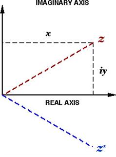
Figure 3.4 Complex plane, spanned by real and imaginary axes. The point representing ![]() is shown along with the complex conjugate
is shown along with the complex conjugate ![]() . Also shown is the modulus
. Also shown is the modulus ![]() .
.
The significance of imaginary and complex numbers can also be understood from a geometric perspective. Consider a number on the positive real axis, say ![]() . This can be transformed by a
. This can be transformed by a ![]() rotation into the corresponding quantity
rotation into the corresponding quantity ![]() on the negative half of the real axis. The rotation is accomplished by multiplying x by −1. More generally, any complex number z can be rotated by
on the negative half of the real axis. The rotation is accomplished by multiplying x by −1. More generally, any complex number z can be rotated by ![]() on the complex plane by multiplying it by
on the complex plane by multiplying it by ![]() , designating the transformation
, designating the transformation ![]() . Consider now a rotation by just
. Consider now a rotation by just ![]() , say counterclockwise. Let us denote this counterclockwise
, say counterclockwise. Let us denote this counterclockwise ![]() rotation by
rotation by ![]() (repress for the moment what i stands for). A second counterclockwise
(repress for the moment what i stands for). A second counterclockwise ![]() rotation then produces the same result as a single
rotation then produces the same result as a single ![]() rotation. We can write this algebraically as
rotation. We can write this algebraically as
![]() (3.77)
(3.77)
which agrees with the previous definition of i in Eqs. (3.71) and (3.72). A ![]() rotation following a counterclockwise
rotation following a counterclockwise ![]() rotation results in the net transformation
rotation results in the net transformation ![]() . Since this is equivalent to a single clockwise
. Since this is equivalent to a single clockwise![]() rotation, we can interpret multiplication by
rotation, we can interpret multiplication by ![]() as this operation. Note that a second clockwise
as this operation. Note that a second clockwise ![]() rotation again produces the same result as a single
rotation again produces the same result as a single ![]() rotation. Thus
rotation. Thus ![]() as well. Evidently
as well. Evidently ![]() . It is conventional, however, to define i as the positive square root of
. It is conventional, however, to define i as the positive square root of ![]() . Counterclockwise
. Counterclockwise ![]() rotation of the complex quantity
rotation of the complex quantity ![]() is expressed algebraically by
is expressed algebraically by
![]() (3.78)
(3.78)
and can be represented graphically as shown in Figure 3.5.
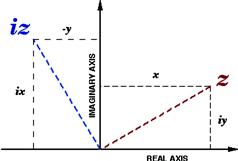
Figure 3.5 Geometric representation of multiplication by ![]() . The point
. The point ![]() is obtained by 90° counterclockwise rotation of
is obtained by 90° counterclockwise rotation of ![]() in the complex plane.
in the complex plane.
Very often we need to transfer a factor i from a denominator to a numerator. The key result is
![]() (3.79)
(3.79)
Several algebraic manipulations with complex numbers are summarized in the following equations:
![]() (3.80)
(3.80)
![]() (3.81)
(3.81)
![]() (3.82)
(3.82)
Note the strategy for expressing a fraction as a sum or real and imaginary parts: multiply by the complex conjugate of the denominator then recognize the square of an absolute value in the form of (3.75).
Problem 3.7.1
Find the real and imaginary parts of ![]() , where
, where ![]() , x and y real.
, x and y real.
Problem 3.7.2
If you don’t mind doing the algebra, analogously find the real and imaginary parts of ![]() .
.
3.8 Factorials, Permutations and Combinations
Imagine that we have a dozen differently colored eggs which we need to arrange in an egg carton. The first egg can go into any one of 12 cups. The second egg can then go into any of the remaining 11 cups. So far, there are ![]() possible arrangements for these two eggs in the carton. The third egg can go into 10 remaining cups. Continuing the placement of eggs, we will wind up with one of a possible total of
possible arrangements for these two eggs in the carton. The third egg can go into 10 remaining cups. Continuing the placement of eggs, we will wind up with one of a possible total of ![]() distinguishable arrangements. (This multiplies out to 479,001,600.) The product of a positive integer n with all the preceding integers down to 1 is called n factorial, designated
distinguishable arrangements. (This multiplies out to 479,001,600.) The product of a positive integer n with all the preceding integers down to 1 is called n factorial, designated ![]() :
:
![]() (3.83)
(3.83)
The first few factorials are ![]() . As you can see, the factorial function increases rather steeply. Our original example involved 12! = 479,001,600. The symbol for factorial is the same as an explanation point. (Thus be careful when you write something like, “To our amazement, the membership grew by 100!”)
. As you can see, the factorial function increases rather steeply. Our original example involved 12! = 479,001,600. The symbol for factorial is the same as an explanation point. (Thus be careful when you write something like, “To our amazement, the membership grew by 100!”)
Can factorials also be defined for nonintegers? Later we will introduce the gamma function, which is a generalization of the factorial. Until then you can savor the amazing result that
![]() (3.84)
(3.84)
Our first example established a fundamental result in combinational algebra: the number of ways of arranging n distinguishable objects (say, with different colors) in n different boxes equals ![]() . Stated another way, the number of possible permutations of n distinguishable objects equals
. Stated another way, the number of possible permutations of n distinguishable objects equals ![]() .
.
Suppose we had started the preceding exercise with just a half-dozen eggs. The number of distinguishable arrangements in our egg carton would then be “only” ![]() . This is equivalent to
. This is equivalent to ![]() . The general result for the number of ways of permuting r distinguishable objects in n different boxes (with
. The general result for the number of ways of permuting r distinguishable objects in n different boxes (with ![]() ) is given by
) is given by
![]() (3.85)
(3.85)
(You might also encounter the alternative notation ![]() , or
, or ![]() .) This formula also subsumes our earlier result, which can be written
.) This formula also subsumes our earlier result, which can be written ![]() . To be consistent with (3.85), we must interpret
. To be consistent with (3.85), we must interpret ![]() .
.
Consider now an alternative scenario in which the eggs are not colored, so that they remain indistinguishable. The different results of our manipulations are now known as combinations. Carrying out an analogous procedure, our first egg can again go into 12 possible cups and the second into one of the remaining 11. But a big difference now is we can no longer tell which is the first egg and which is the second—remember they are indistinguishable. So the number of possibilities is reduced to ![]() . After placing 3 eggs in
. After placing 3 eggs in ![]() available cups, the identical appearance of the eggs reduces the number of distinguishable arrangements by a factor of
available cups, the identical appearance of the eggs reduces the number of distinguishable arrangements by a factor of ![]() . We should now be able to generalize for the number of combinations with m indistinguishable objects in n boxes. The result is
. We should now be able to generalize for the number of combinations with m indistinguishable objects in n boxes. The result is
![]() (3.86)
(3.86)
Another way of deducing this result. The total number of permutations of n objects is, as we have seen, equal to ![]() . Now, permutations can be of two types: indistinguishable and distinguishable. The eggs have
. Now, permutations can be of two types: indistinguishable and distinguishable. The eggs have ![]() indistinguishable permutations among themselves, while the empty cups have
indistinguishable permutations among themselves, while the empty cups have ![]() indistinguishable ways of hypothetically numbering them. Every other rearrangement is distinguishable. If
indistinguishable ways of hypothetically numbering them. Every other rearrangement is distinguishable. If ![]() represents the total number of distinguishable configurations then
represents the total number of distinguishable configurations then
![]() (3.87)
(3.87)
which is equivalent to (3.86).
A simple generalization to distinguish permutations from combinations is that permutations are for lists, in which the order matters, while combinations are for groups in which the order doesn’t matter.
Suppose you have n good friends seated around a dinner table who wish to toast one another by clinking wineglasses. How many “clinks” will you hear? The answer is the number of possible combinations of objects taken 2 at a time from a total of n, given by
![]() (3.88)
(3.88)
You can also deduce this more directly by the following argument. Each of n diners clinks wineglasses with his or her ![]() companions. You might first think there must be
companions. You might first think there must be ![]() clinks. But, if you listen carefully, you will realize that this counts each clink twice, one for each clinkee. Thus dividing by 2 gives the correct result
clinks. But, if you listen carefully, you will realize that this counts each clink twice, one for each clinkee. Thus dividing by 2 gives the correct result ![]() .
.
3.9 The Binomial Theorem
Let us begin with an exercise in experimental algebra:
 (3.89)
The array of numerical coefficients in (3.89)
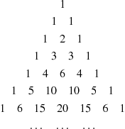 (3.90)
is called Pascal’s triangle. Note that every entry can be obtained by taking the sum of the two numbers diagonally above it, e.g. 15 = 5 + 10. These numbers are called binomial coefficients. You can convince yourself that they are given by the same combinatorial formula as ![]() in Eq. (3.86). The binomial coefficients are usually written
in Eq. (3.86). The binomial coefficients are usually written ![]() . Thus
. Thus
![]() (3.91)
(3.91)
where each value of n, beginning with 0, determines a row in the Pascal triangle.
Setting ![]() , the binomial formula can be expressed
, the binomial formula can be expressed
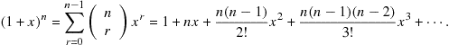 (3.92)
This was first derived by Isaac Newton in 1666. Remarkably, the binomial formula is also valid for negative, fractional, and even complex values of n, which was proved by Niels Henrik Abel in 1826. (It is joked that Newton didn’t prove the binomial theorem for noninteger n because he wasn’t Abel.) Here are a few interesting binomial expansions which you can work out for yourself:
![]() (3.93)
(3.93)
![]() (3.94)
(3.94)
![]() (3.95)
(3.95)
Each of the above series is convergent only for ![]() .
.
Problem 3.9.1
Determine the first few terms in the expansion of ![]() .
.
3.10 e is for Euler
Imagine there is a bank in your town that offers you 100% annual interest on your deposit (we will let pass the possibility that the bank might be engaged in questionable loan-sharking activities). This means that if you deposit $1 on January 1, you will get back $2 one year later. Another bank across town wants to get in on the action and offers 100% annual interest compounded semiannually. This means that you get 50% interest credited after half a year, so that your account is worth $1.50 on July 1. But this total amount then grows by another 50% in the second half of the year. This gets you, after 1 year,
![]() (3.96)
(3.96)
A third bank picks up on the idea and offers to compound your money quarterly. Your $1 there would grow after a year to
![]() (3.97)
(3.97)
Competition continues to drive banks to offer better and better compounding options, until the Eulergenossenschaftsbank apparently blows away all the competition by offering to compound your interest continuously—every second of every day! Let’s calculate what your dollar would be worth there after 1 year. Generalization from Eq. (3.97) suggests that compounding n times a year produces ![]() . Here are some numerical values for increasing n:
. Here are some numerical values for increasing n:
![]() (3.98)
(3.98)
The ultimate result is
![]() (3.99)
(3.99)
This number was designated e by the great Swiss mathematician Leonhard Euler (possibly after himself). Euler (pronounced approximately like “oiler”) also first introduced the symbols i, ![]() , and
, and ![]() . After
. After ![]() itself, e is probably the most famous transcendental number, also with a never-ending decimal expansion. The tantalizing repetition of “1828” is just coincidental.
itself, e is probably the most famous transcendental number, also with a never-ending decimal expansion. The tantalizing repetition of “1828” is just coincidental.
The binomial expansion applied to the expression for e gives
![]() (3.100)
(3.100)
As ![]() , the factors
, the factors ![]() all become insignificantly different from n. This suggests the infinite-series representation for e
all become insignificantly different from n. This suggests the infinite-series representation for e
![]() (3.101)
(3.101)
Remember that ![]() and
and ![]() . This summation converges much more rapidly than the procedure of Eq. (3.99). After just six terms, we obtain the approximate value
. This summation converges much more rapidly than the procedure of Eq. (3.99). After just six terms, we obtain the approximate value ![]() .
.
Let’s return to consideration of interest-bearing savings accounts, this time in more reputable banks. Suppose a bank offers X% annual interest. If ![]() , your money would grows by a factor of
, your money would grows by a factor of ![]() every year, without compounding. If we were able to get interest compounding n times a year, the net annual return would increase by a factor
every year, without compounding. If we were able to get interest compounding n times a year, the net annual return would increase by a factor
![]() (3.102)
(3.102)
Note that, after defining ![]() ,
,
![]() (3.103)
(3.103)
Therefore, in the limit ![]() , Eq. (3.102) implies the series
, Eq. (3.102) implies the series
![]() (3.104)
(3.104)
This defines the exponential function, which plays a major role in applied mathematics. The very steep growth of the factorials guarantees that the expansion will converge to a finite quantity for any finite value of x, real, imaginary, or complex. The inverse of the exponential function is the natural logarithm, defined in Eq. (3.55):
![]() (3.105)
(3.105)
Two handy relations are
![]() (3.106)
(3.106)
When the exponent of the exponential is a complicated function, it is easier to write
![]() (3.107)
(3.107)
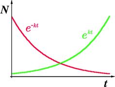
Exponential growth and exponential decay, sketched in Figure 3.6, are observed in a multitude of natural processes. For example, the population of a colony of bacteria, given unlimited nutrition, will grow exponentially in time:
![]() (3.108)
(3.108)
where ![]() is the population at time
is the population at time ![]() and k is a measure of the rate of growth. Conversely, a sample of a radioactive element will decay exponentially:
and k is a measure of the rate of growth. Conversely, a sample of a radioactive element will decay exponentially:
![]() (3.109)
(3.109)
A measure of the rate of radioactive decay is the half-life![]() , the time it takes for half of its atoms to disintegrate. The half-life can be related to the decay constant k by noting that after time
, the time it takes for half of its atoms to disintegrate. The half-life can be related to the decay constant k by noting that after time ![]() ,
, ![]() is reduced to
is reduced to ![]() . Therefore
. Therefore
![]() (3.110)
(3.110)
and, after taking natural logarithms,
![]() (3.111)
(3.111)
No doubt, many of you will become fabulously rich in the future, due, in no small part, to the mathematical knowledge we are helping you acquire. You will probably want to keep a small fraction of your fortune in some CDs at your local bank. In better economic times there was a well-known “Rule of 72” which stated that to find the number of years required to double your principal at a given interest rate, just divide 72 by the interest rate. For example, at 8% interest, it would take about ![]() . To derive this rule, assume that the principal
. To derive this rule, assume that the principal ![]() will increase at an interest rate of
will increase at an interest rate of ![]() to
to ![]() in Y years, compounded annually. Thus
in Y years, compounded annually. Thus
![]() (3.112)
(3.112)
Taking natural logarithms we can solve for
![]() (3.113)
(3.113)
To get this into a neat approximate form ![]() , let
, let
![]() (3.114)
(3.114)
You can then show for interest rates in the neighborhood of 8% (![]() ), the approximation will then work with the constant approximated by 72.
), the approximation will then work with the constant approximated by 72.