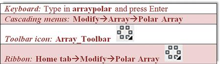
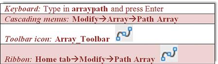
Polar, Rectangular, and Path Arrays
Learning Objectives
In this chapter, we introduce the concept of an array and discuss the following:
![]() Object, center, quantity, and degrees
Object, center, quantity, and degrees
![]() Additional operations with polar arrays
Additional operations with polar arrays
![]() Object, rows and columns, and distances
Object, rows and columns, and distances
At the end of this chapter you will be able to create polar, rectangular, and path arrays. You will then start a new in-class mechanical project.
Estimated time for completion of chapter (lesson and project): 3 hours.
Arrays are very useful tools in AutoCAD to create patterns of objects. These patterns can be of a circular, linear, or path type, hence the polar array, rectangular array, and path array discussions that follow. In a strict sense, these tools are not something entirely new but merely automate what you can do (albeit tediously) by regular commands learned in Chapter 1, and they are huge time savers.
The array command underwent a major rework in AutoCAD 2012, with some additional minor enhancements for 2013 and 2014. If you are using this textbook to refresh your skills and have used older versions of AutoCAD, you are in for a surprise. Not only has an entirely new type of array been added (path array), but the tool is now command-line activated, with the Ribbon assisting with modifications, or almost entirely Ribbon driven. For better or for worse, the familiar Array dialog box is gone, and a whole new set of possibilities is opened up.
This chapter introduces the various arrays by assuming that the student is new to AutoCAD and has never used or seen the older, legacy, version of the command. It is, however, referred to and described, just in case you end up using a pre-2012 AutoCAD at some point in the future.
8.1 Polar Array
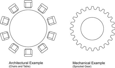
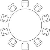
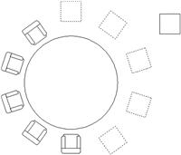
A polar array is a collection of objects around some common point arranged in a circle (or part thereof). An example in architecture is a group of chairs arranged around a circular table. The idea is to draw the table, then one chair, and after positioning the chair exactly where it will be in relation to the table, use a polar array to copy it around the table to create, let us say, ten of them. The array command copies and rotates them into position and spaces them out evenly, a task that would have taken a while to do one chair at a time.
In mechanical engineering, an example may be the teeth of a sprocket gear. You draw the circle representing the wheel of the gear; put in one tooth properly drawn, detailed, and centered on top; then array to get the full gear. Figure 8.1 shows illustrations of what was just discussed. There are, of course, many other examples.
Steps in Creating a Polar Array
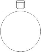
First of all, we need to create something to array. So go ahead and draw a circle of any size to represent the table just discussed, then create a convincing-looking chair. You may want to make a block out of it after you are done for convenience.
Next, position the chair at the top of the table, as seen in Figure 8.2. Be sure to line it up perfectly on the vertical axis, or else the array will be skewed off center; and move it back a bit from the table with Ortho on. What does AutoCAD need to know to do the array? The following four items are critical to a polar array; although note that only the first two items are explicitly asked for by AutoCAD as you create the array:
![]() It needs to know what object(s) to array (that would be the chair, not the table).
It needs to know what object(s) to array (that would be the chair, not the table).
![]() It needs to know the center point of the array (center of the table).
It needs to know the center point of the array (center of the table).
![]() It needs to know how many objects to create (let us stick to ten or so).
It needs to know how many objects to create (let us stick to ten or so).
![]() It needs to know if the pattern goes all the way around (that is, is it 360° or less).
It needs to know if the pattern goes all the way around (that is, is it 360° or less).
It is useful to memorize these steps and realize what you need to do before even starting up the array command; that way you have a clear idea of what to do and what data to enter as you get going. Once you have the table and chair drawn, follow the steps shown to create the polar array.
Step 1. Start up the array command via any of the preceding methods (it is recommended to have the Ribbon turned on).
Step 2. Select the chair block.
![]() AutoCAD says: Type=Polar Associative=Yes
AutoCAD says: Type=Polar Associative=Yes
Specify center point of array or [Base point/Axis of rotation]:
Step 4. You successfully selected the object to array. You now need to specify the center point of the array. Simply select the center of the large circle (the table) using the CENter OSNAP. AutoCAD creates a set of chairs around the table.
![]() AutoCAD says: Enter elect grip to edit array or [ASsociative/Base point/Items/Angle between/Fill angle/ROWs/Levels/ROTate items/eXit]<eXit>:
AutoCAD says: Enter elect grip to edit array or [ASsociative/Base point/Items/Angle between/Fill angle/ROWs/Levels/ROTate items/eXit]<eXit>:
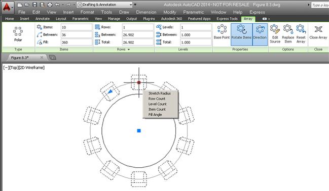
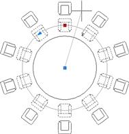
Step 5. Note a few things at this point. The array is automatically associative (look for that button to be active in the Ribbon). This means all the pieces are linked and not separate, a very desirable new property of arrays. Also note the details shown in the Ribbon. Here, you can modify the number of items (chairs), and the angle to fill under the Items tab. Make sure you have ten chairs for this exercise.
Step 6. Your array is essentially done, so just press Enter to accept. If you wish, experiment with some of the variables such as Fill and Between. Also note how the chairs are rotated to face the table via the Rotate Items button that was automatically set (under Properties tab). You can, of course, turn that feature off. The completed polar array is shown in Figure 8.3.
Additional Operations with Polar Array
Your new array behaves like a block (assuming Associative is set), a major difference first introduced in AutoCAD 2012, prior to which the new pieces of the array were not connected in any way. Click on one of the chairs with your mouse and it becomes selected, with several varieties of grips visible. If you hover your mouse over the chair grip, you see a menu of additional options. Finally, a new Ribbon Array tab appears. All are seen in Figure 8.4. Let us take a closer look at the Ribbon and the Grip menu.
The Ribbon has two areas of interest, the Items category and the Options category, as seen in Figure 8.5. The Items category we already mentioned and it is relatively self-explanatory. Top to bottom, the first value (10) is the number of items in the array, and you can change it for an instant update. Below that is the angle between all the objects (36°), and finally, below that, the total angle filled (360°, or a full circle). This should make sense as 36×10=360.
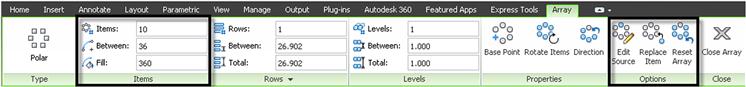
The Options category’s tools are a bit more involved. They are described next:
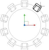
![]() Edit Source. This option allows you to edit and modify the source object. These changes are then reflected in the overall array. If you forget which object was the original source, it does not matter; you can pick any of the chairs and work on it. Execute the command, select the object, modify it, and when done, type in arrayclose. Figure 8.6 shows Edit Source in progress.
Edit Source. This option allows you to edit and modify the source object. These changes are then reflected in the overall array. If you forget which object was the original source, it does not matter; you can pick any of the chairs and work on it. Execute the command, select the object, modify it, and when done, type in arrayclose. Figure 8.6 shows Edit Source in progress.
![]() Replace Item. If editing the source is too time consuming, then just replace it with another design via this option. AutoCAD asks you to select the replacement object and a base point. Use the Key Point option to pick a point on the replacement object. Finally, select an item (or several items) in the array to replace. Figure 8.7 shows Replace Item in action as squares replace the chair symbol.
Replace Item. If editing the source is too time consuming, then just replace it with another design via this option. AutoCAD asks you to select the replacement object and a base point. Use the Key Point option to pick a point on the replacement object. Finally, select an item (or several items) in the array to replace. Figure 8.7 shows Replace Item in action as squares replace the chair symbol.
![]() Reset Array. This is an easy one. Autodesk figured you will mess up a few arrays while learning this tool (speaking from experience, of course) and included a Reset button. Its function is apparent immediately on use.
Reset Array. This is an easy one. Autodesk figured you will mess up a few arrays while learning this tool (speaking from experience, of course) and included a Reset button. Its function is apparent immediately on use.
Next, we have the menu seen when the mouse is held over the chair grip. Run through all the options as you read the descriptions. It contains the following tools:
![]() Stretch Radius. This option simply expands the radius of the overall array. The effect is the same as if you just activate the grip and move the mouse. Stretch Radius in action is seen in Figure 8.8.
Stretch Radius. This option simply expands the radius of the overall array. The effect is the same as if you just activate the grip and move the mouse. Stretch Radius in action is seen in Figure 8.8.
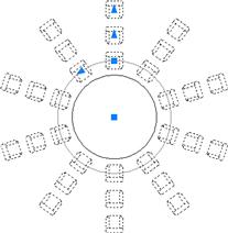
![]() Row Count. This option adds another set of row(s) of items in front or behind the main row, as seen in Figure 8.9.
Row Count. This option adds another set of row(s) of items in front or behind the main row, as seen in Figure 8.9.
![]() Level Count. This option adds 3D levels and its discussion is not be included in this 2D-only chapter.
Level Count. This option adds 3D levels and its discussion is not be included in this 2D-only chapter.
![]() Item Count. This option adds or deletes items (similar to the Ribbon function), or it can just be used to tell you how many items there are in the array, also a useful feature.
Item Count. This option adds or deletes items (similar to the Ribbon function), or it can just be used to tell you how many items there are in the array, also a useful feature.
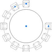
![]() Fill Angle. This option (also via the triangle grip) changes the included angle, currently set to 360°. An example is shown in Figure 8.10, where the fill angle has been rolled back to 270°.
Fill Angle. This option (also via the triangle grip) changes the included angle, currently set to 360°. An example is shown in Figure 8.10, where the fill angle has been rolled back to 270°.
Go over all these features until you are comfortable working with them. Be aware that you also can explode the array, which makes it behave like the “legacy” array, where each piece is separate. A short discussion of the legacy tools follows.
Legacy Polar Array (Pre-AutoCAD 2012)
Because the array command was so heavily redesigned for the 2012 release of AutoCAD, it makes sense to briefly mention the legacy polar array tool encountered via a dialog box prior to that release. If you have AutoCAD 2011 or any of the older versions, then the polar array can be accessed by typing in array and pressing Enter, or using the usual toolbar, cascading menus, or Ribbon (if available) methods.
What you then see is the classic Array dialog box (Figure 8.11, taken from AutoCAD 2011). You first need to make sure you have selected the Polar Array radio button at the very top. Then, run through the same steps outlined in the beginning of this chapter and shown here again:
![]() Select object to array (button at top right).
Select object to array (button at top right).
![]() Select the center point of the array (button center top right).
Select the center point of the array (button center top right).
![]() Enter how many objects to create (in the middle).
Enter how many objects to create (in the middle).
![]() Enter how many degrees to fill (just below the previous entry).
Enter how many degrees to fill (just below the previous entry).
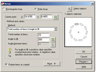
Preview the array via the Preview<button and press OK to finish off the array.
Note that the entire array is not a block, just a collection of objects, and to redo the whole thing, you need to erase all the copies, leaving just the table and the original chair, then repeat everything. That is why the Preview button is so important. Do not be so quick to press OK. This array, of course, has none of the editing options introduced in AutoCAD 2012.
8.2 Rectangular Array
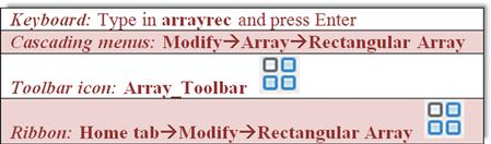
The idea behind a rectangular array is not fundamentally different from a polar one. We are looking to replicate objects, but this time in rows (horizontal) and columns (vertical). In 3D, you can also do levels, which we do not address here. An example, as shown in Figure 8.12, may be columns of a warehouse. If they are spread out evenly, then this is the perfect tool for this. You simply draw one I-beam column, make a block out of it, and array it up and across the appropriate area.
Steps in Creating a Rectangular Array
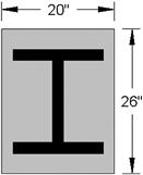
The first thing to do is to draw a convincing-looking I-beam. Because we need actual distances, you cannot just randomly draw any object; use known sizing this time around. With one of the columns in Figure 8.12 as a model, create a 20" wide by 26" tall rectangle. Inside of it, put an I-beam drawn with basic linework and a solid hatch fill, and shade the background a light gray (Figure 8.13). Finally, make a block out of it. That sets up the column for an array.
Now, what does AutoCAD need to know to create a rectangular array? The following three items are critical to a rectangular array; although, note that only the first item is explicitly asked for by AutoCAD as you create the array:
![]() It needs to know what object(s) to array (the I-beam column).
It needs to know what object(s) to array (the I-beam column).
![]() It needs to know how many rows and columns to create (rows=across, columns=up and down).
It needs to know how many rows and columns to create (rows=across, columns=up and down).
![]() It needs to know the distance between the rows and the columns (from centerline to centerline).
It needs to know the distance between the rows and the columns (from centerline to centerline).
Step 1. Start up the array command via any of the preceding methods (it is recommended to have the Ribbon turned on).
Step 2. Select the I-beam column block.
Step 3. Press Enter. A small array of items are created, with grips visible.
![]() AutoCAD says: Type=Rectangular Associative=Yes
AutoCAD says: Type=Rectangular Associative=Yes
Select grip to edit array or [ASsociative/Base point/COUnt/Spacing/ COLumns/Rows/Levels/eXit]<eXit>:
Step 4. You have now successfully created the basic rectangular array. You still need to define the exact number of rows and columns, however, as well as the distance between them, as this current array is rather arbitrary. You can do this either via command line, dynamically (using grips), or via the Ribbon. Figure 8.14 shows how you can pull the items diagonally in a dynamic fashion using the center grip. You can also do this via the outer arrow grips. This dynamic method is not really appropriate for setting distances between the columns, which are random values for now, but it does make creating the pattern very easy.
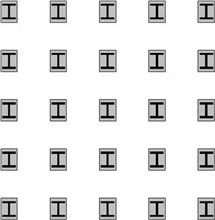
Step 5. If you have the Ribbon up, then you just enter values. We want to create a 5×5 array, so start by entering those values into the Ribbon’s “Columns:” and “Rows:” fields. For distances between the columns use the value 72.
Step 6. If using the command line, you just have to follow the prompts for Columns, Rows, and Spacing. Regardless of which you start with (Rows or Columns), AutoCAD asks you for the spacing as needed. Press Enter when done. Your rectangular array should look like Figure 8.12.
Additional Operations with Rectangular Array
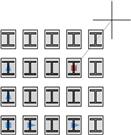
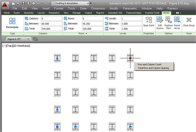
After a lengthy discussion on additional operations with the polar array, you will find these options with the rectangular array to be quite familiar. Click on the new array of I-beam columns, and notice a set of grips, a menu, and an Array tab in the Ribbon, all similar to the earlier polar array (Figure 8.15).
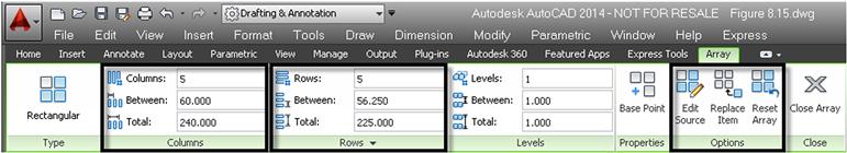
The Ribbon has three areas of interest this time: the Columns, Rows, and Options categories, as seen in Figure 8.16. The Columns category allows you to adjust the number of columns, distance between them, and the total distance. The Rows category is the exact same thing but for rows. Finally, in the Options category, we already discussed the functionality of Edit Source, Replace Item, and Reset Array. They are all exactly the same as with the polar array.
Next, we have the menu seen when the mouse is held over the top right I-beam column grip. The two choices are Row and Column Count and Total Row and Column Spacing. Their functions should be relatively easy to see by just trying them out. If you activate the first choice and move the mouse, the number of rows and columns increases, but the spacing remains the same. If you activate the second choice, the spacing increases but not the number of rows and columns.
Finally, try out the other grips on the array, specifically the ones in the lower left corner. You find that the square grip moves the entire array and the inner triangles increase the spacing. The outer triangle grips (toward the edges of the array), however, are used to increase the count. Experiment with all the options.
Legacy Rectangular Array (Pre-AutoCAD 2012)
The legacy rectangular array is accessed via the same methods as the legacy polar array. When the dialog box appears, make sure the Rectangular array radio button is selected and you see what is shown in Figure 8.17 (also taken from AutoCAD 2011). The procedure remains basically the same. You must select the object, then enter the number of rows and columns, followed by the distances between those rows and columns. Do a preview and press OK.
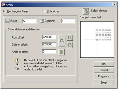
Note again that the entire array is not a block, just a collection of objects; and to redo the whole thing, you need to erase all the copies, leaving just one I-beam column and repeat everything. This array, of course, has none of the editing options introduced in AutoCAD 2012 either.
In general, polar arrays are used more often than the rectangular ones, but both are important to know.
8.3 Path Array
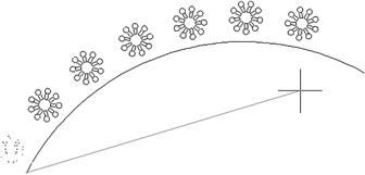
The path array is the new kid on the block. Requested by users, this feature was finally added in AutoCAD 2012. The idea is simple, and it is surprising that this feature was not added earlier. A path array creates a pattern along any predetermined pathway, of any shape, as opposed to a strictly circular or linear one. This path can be an arc, a pline, or a spline. Because plines and splines have not yet been discussed (a Chapter 11 topic), we focus on arcs as the pathways. A path array can also be created in 3D, but we do not get into that right now. An example of a path array in progress is shown in Figure 8.18.
Steps in Creating a Path Array
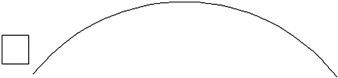
Boiled down to its essence, the path array just needs an object to array and a path to follow. Much like the previous two arrays, the objects can be spread out dynamically with mouse movements (as seen being done in Figure 8.19) or with an input of a specific value. All other options flow from this basic approach. Let us give it a try. Create an arc and some random object to array; a rectangle will do, as seen in Figure 8.19.
So, what does AutoCAD need to know to do the array?
![]() It needs to know what object(s) to array (the rectangle).
It needs to know what object(s) to array (the rectangle).
![]() It needs to know the path (the arc).
It needs to know the path (the arc).
![]() It needs to know how many objects to create (let us stick to ten or so).
It needs to know how many objects to create (let us stick to ten or so).
Step 1. Start up the array command via any of the preceding methods.
![]() AutoCAD says: Type=Path Associative=Yes
AutoCAD says: Type=Path Associative=Yes
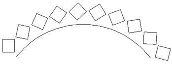
Step 4. You successfully selected the object to array. Now, select the path by clicking on the arc. A number of copies of the rectangle appear along the arc.
![]() AutoCAD says: Select grip to edit array or [ASsociative/Method/Base point/Tangent direction/Items/Rows/Levels/Align items/Z direction/eXit]<eXit>:
AutoCAD says: Select grip to edit array or [ASsociative/Method/Base point/Tangent direction/Items/Rows/Levels/Align items/Z direction/eXit]<eXit>:
Step 5. You have essentially created the basic path array, but you can do a tremendous amount of modification to this basic layout. The easiest way to modify it is via the Ribbon. Under the Items tab you have the most basic of the “mods,” such as total number of items and the distance between them. Also note how you can alter the path array via dynamic movement of the grips. Be sure to keep the array associative, as with the previous examples. The completed array is seen in Figure 8.20.
Additional Operations with Path Array
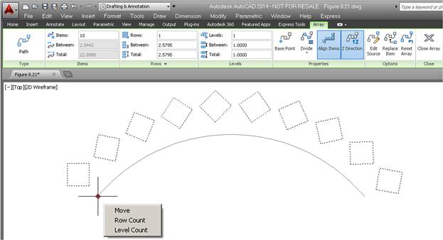
Just as with the previous two arrays, the path array has its own Ribbon tab, which is revealed by selecting one of the elements in the array, as well as its own menu, revealed as you hover the mouse over the grip, as seen in Figure 8.21.
The Items category is of some interest and at this point should be familiar. You can vary the number of elements, distances between them, and total distance. Under the Properties category experiment with redefining the base point—this shifts your pattern around. Also check out Align Items—this makes all your elements face the same direction versus angling with the curve. Edit Source, Replace Item, and Reset Array all have the same meanings as with the previous polar and rectangular arrays. Spend a few moments understanding the cause and effect of these options.
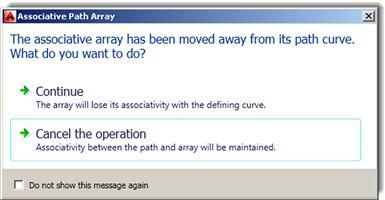
Finally, let us take a look at the grip menu. It also should be more familiar after your experiences with the previous two arrays. Move moves the array away from its originating path and triggers a warning along the way (Figure 8.22). You may have seen the warning with earlier arrays as well, if you tried to move them around. Simply press Continue and carry on.
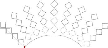
Row Count creates additional rows of the pattern, as seen in Figure 8.23. This option also repeats what is available with the other arrays. Level Count is not covered here, as it is a 3D function.
8.4 In-Class Drawing Project: Mechanical Device
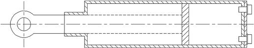
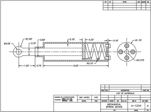
Let us now put what you learned to use by drawing a mechanical gadget (a suspension strut of sorts), created years ago for a class. Although what it is exactly is still debatable, the gadget proved to be an excellent drawing example and features quite a bit of what we covered in this and preceding chapters as well as a few minor nuances of AutoCAD drafting that, once learned, raise your skill levels considerably. The trick is to make your drawing look exactly like the example. If you approximate and cut corners, you miss out on some of the important concepts that give a more professional look to your drawings.
A full-page view of the completed device is found toward the end of the chapter, see Figure 8.33. Take a good look at it and decide on a strategy to draw it. Over the course of the next few pages, you will see a step-by-step process to actually do it. Follow the steps carefully, and do not worry about the thick border; that is a polyline, to be covered in Level 2. The title block is otherwise just a simple collection of lines and text.
Step 1. For starters open a new file, give it a name (Save As…), and set up your layers. We need, at a minimum,
M-Part, Color: Green (for most of the parts of the device).
M-Dims, Color: Cyan (for the dimensions).
M-Hidden, Color: Yellow, Linetype: Hidden (for all hidden lines).
M-Center, Color: Red, Linetype: Center (for the main centerlines).
M-Hatch, Color: 9 (a gray for cross-section cutaways).
You may also want additional layers for the spring and the title block. You can decide on the exact layers and their colors; the preceding is just a guide. Also, the images in this chapter remain black and white, for clarity on a white page.
Step 2. Set up all the necessary items for smooth drafting, such as the Text Style (Arial, .20), the Dim Style, and Units (either Architectural or Mechanical is fine), and get rid of the UCS icon if you do not like it.
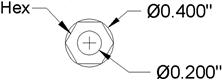
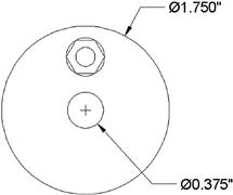
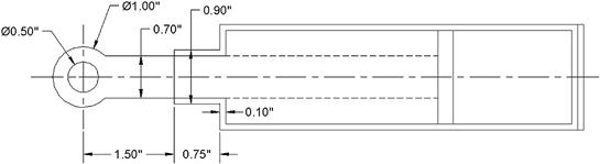
Step 3. To begin the drawing itself, we need to start with the hex bolts. Go ahead and draw one of them according to the information in Figure 8.24. Be very careful, all sizes are diameters not radiuses; you must tell AutoCAD this by pressing d for Diameter while making a circle. This has tripped up many students in the past. Also do not forget to make layer M-Part current. If the bolt is anything but green in color, you missed this step. The dimensions are only for your reference for now; there is no need to draw them.
Step 4. Now make a block out of the bolt, calling it Bolt - Top View.
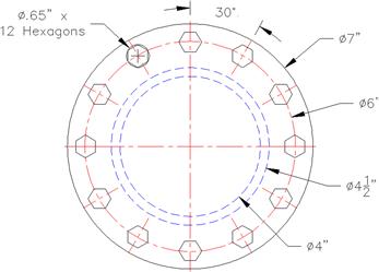
Step 5. Complete the rest of the top view by drawing the remaining circles and positioning the bolt at the top, as shown in Figure 8.25. Use accuracy (OSNAPs), although the bolt can be any distance from the top of the circle. Be careful to use diameter, as indicated.
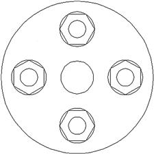
Step 6. Array the bolt around the top view four times, as shown in Figure 8.26.
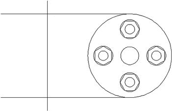
Step 7. You now have to project the main body of the part based on this top view. The best way is by drawing two horizontal guidelines, of any length, starting from the top and bottom quadrants of the big circle; then draw an arbitrary vertical line to mark the beginning of the part on the right, as shown in Figure 8.27.
Step 8. Trim or fillet the main vertical guideline and continue offsetting, based on the given geometry, to “sketch out” the basic outline of the shape, as seen in Figure 8.28. Do not yet add dimensions; they are for construction only.
Step 9. Continue adding the basic geometry to the side view, as well as hidden and centerlines, as shown in Figure 8.29. Set LTSCALE to .4.
Step 10. Add the bolt projections, as seen in Figure 8.30 (the depth into the side view can be approximated). Finally, add hatch patterns, using the Angle option to reverse the hatch directions, which is a common technique in mechanical design to differentiate the parts from each other in a cross section.
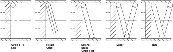
Step 11. Now, how do you do the spring? Well, this is where the Circle/TTR comes in. Although we have not practiced this version of the circle command, it is very simple to do. Start it up and select the TTR option. Then, pick the vertical and the horizontal lines where the circle needs to go (seen in Figure 8.31) and specify a radius (0.10"). One way of proceeding is to draw a straight arbitrary line down from the center of that circle, rotate the line 15° about that center point, then offset 0.1" in each direction, erase the original line, extend the two new ones to the bottom (if necessary), and repeat the process, as seen in Figure 8.31. Once a set is done, you can mirror the rest and trim carefully to create the impression of a coiled spring.
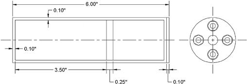
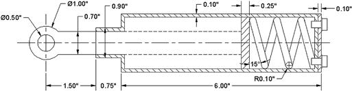
Step 12. Finally, add dimensions (Figure 8.32) and a title block (Figure 8.33) by use of rectangles. The title block and its contents are typical of a mechanical engineering drawing.
Summary
You should understand and know how to use the following concepts and commands before moving on to Chapter 9:
![]() Additional operations and options
Additional operations and options
![]() Distance between rows and columns
Distance between rows and columns
Exercises
1. In a new file, draw this slightly altered version of the image found at the opening of this chapter, shown here with all the necessary dimensions. (Difficulty level: Easy; Time to completion: 10 minutes.)
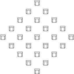
2. In a new file, draw the following five row by five column rectangular array. The chairs are 20" by 20" and the offset between them is 50". The array is also at a 45° angle. (Difficulty level: Easy; Time to completion:<10 minutes.)
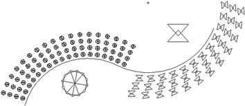
3. In a new file, draw the following set of path arrays. The two paths are simple arcs, and the symbols used are scaled up and shown next to the patterns. (Difficulty level: Easy; Time to completion:<10 minutes.)
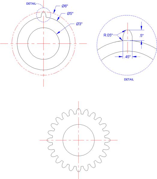
4. In a new file, draw the following gear array. Begin with circles of the indicated diameter. Then, focus on creating the first tooth, as seen in the detail. Make sure it is centered and aligned. Finally, array the tooth (24 teeth are used in the example) and clean up the design with trimming. The final result follows. (Difficulty level: Moderate; Time to completion:<20 minutes.)
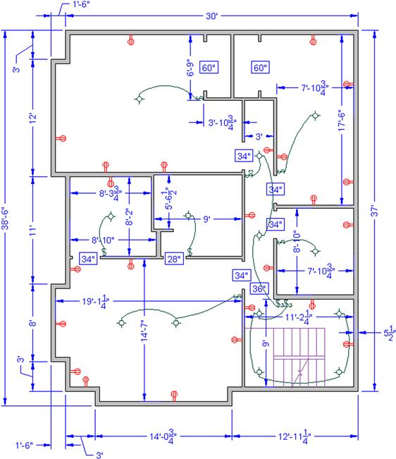
5. The final exercise of this chapter has no arrays but is a basic floor plan to keep your drawing skills sharp. It also features some electrical symbol blocks; get used to them, as they are standard in any electrical layout. The numbers inside the rectangles are the doorway dimensions. All walls are 5½". A few secondary dimensions are not given due to space limitations; you need to make a best estimate. Use proper layers and make a block of all the electrical symbols. (Difficulty level: Moderate; Time to completion: 90–120 minutes.)