Advanced Design and File Management Tools
Learning Objectives
In this chapter, we continue to introduce a variety of advanced tools and discuss the following:
By the end of the chapter, you will add significantly to your command repertoire.
Estimated time for completion of chapter: 3 hours.
15.1 Introduction to Advanced Design and File Management Tools
This is easily the most diverse and unique chapter you will read in the book. Here, we really explore the “nooks and crannies” of AutoCAD and cover a wide range of very diverse commands. The reason these particular commands are grouped here is because this text was written from the start to simplify and isolate core topics and essential ideas, without cluttering the main themes with additional AutoCAD commands and concepts. Several more “big ideas” are left, such as xrefs, attributes, and isometrics. Those are addressed in upcoming chapters. However, that leaves out a great deal of useful concepts and commands that did not quite fit in anywhere else.
These bite-sized chunks of information form the basis of this chapter. Many of these topics are just random commands, standing alone, not part of any other major concept, while some may be part of a larger family but were not included earlier to avoid getting distracted from a much more important theme. All are useful to one extent or another and are necessary for a well-rounded knowledge of AutoCAD.
Obviously, this is not an exhaustive list; some items have been left out due to space limitations, but for the most part, the important ones are here. The list is in alphabetical order. Go through it at your own pace, noting how each concept or command can help you in your design work. Some are whimsical, some are rather odd, and surely you will find one or two that you cannot do without!
15.2 Align
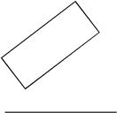
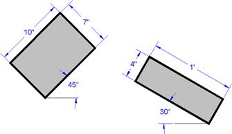
This command does exactly what it advertises, aligns one object to another. In Figure 15.1, we have a rectangle drawn and rotated to some random angle and below it a straight line. While one can always measure the angle of the rectangle relative to the line and use the rotate command, there is a much easier and accurate way to align the rectangle to the line (or vice versa).
Step 1. Type in align and press Enter. You can also use the cascading menus Modify→3D Operations→Align. There are no toolbar or Ribbon equivalents.
Step 2. Select the object to be moved into alignment (the rectangle). Press Enter.
![]() AutoCAD says: Specify first source point:
AutoCAD says: Specify first source point:
Step 3. Pick the lower left corner of the rectangle using the ENDpoint OSNAP (point 1 in Figure 15.2).
![]() AutoCAD says: Specify first destination point:
AutoCAD says: Specify first destination point:
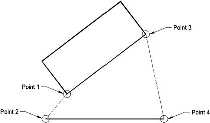
Step 4. Pick the left point of the line using the ENDpoint OSNAP (point 2 in Figure 15.2).
![]() AutoCAD says: Specify second source point:
AutoCAD says: Specify second source point:
Step 5. Pick the lower right corner of the rectangle using the endpoint OSNAP (point 3 in Figure 15.2).
![]() AutoCAD says: Specify second destination point:
AutoCAD says: Specify second destination point:
Step 6. Pick the right point of the line using the ENDpoint OSNAP (point 4 in Figure 15.2).
![]() AutoCAD says: Specify third source point or<continue>:
AutoCAD says: Specify third source point or<continue>:
Step 7. You have no need for a third set of points, so press Enter.
![]() AutoCAD says: Scale objects based on alignment points? [Yes/No]<N>:
AutoCAD says: Scale objects based on alignment points? [Yes/No]<N>:
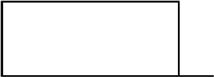
You can do something interesting here. Not only can you align the rectangle to the line, you can also scale it up to the line if needed by selecting Yes. We do not try this now but go back after learning the basic align command and try this variation of it. For now, just press Enter to accept the default No option. The rectangle is aligned to the line, as seen in Figure 15.3.
15.3 Action Recording
Action recording is a relatively new tool in AutoCAD that is used to build Action Macros and save them as *.actm files. Macros is short for macroinstructions, a computer term that can be defined as a short set of instructions to perform a task. The idea here is to actually record your on-screen actions and save them for future use. Needless to say, these actions should be some sort of useful steps to build a tedious or repetitive object and not just any simple steps. You can then use this macro to make your life easier later on. The technique can be applied in both 2D and 3D.
To give this a try, open up a brand-new file with the Ribbon present. You can use the command without the Ribbon, by simply typing in actrecord to start the process and stop to end it, but it’s easier and more visual with the Ribbon present. Then start the command via any of the following methods:
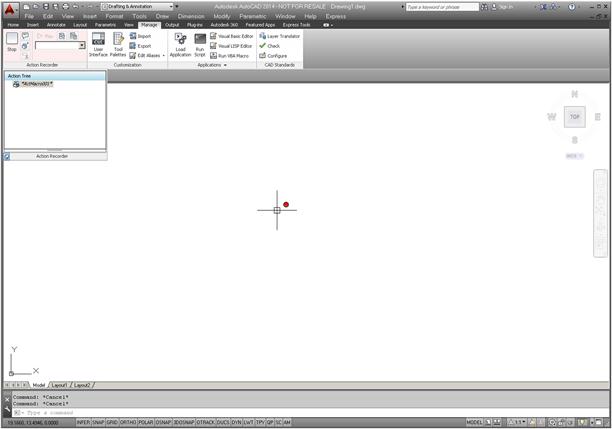
You then see what is shown in Figure 15.4. Notice the Ribbon tab on the left has turned light pink and the record button became a stop button. The mouse has also acquired a red “Recording” dot. If for any reason the Ribbon did not open to the right tab, just manually select the Manage tab.
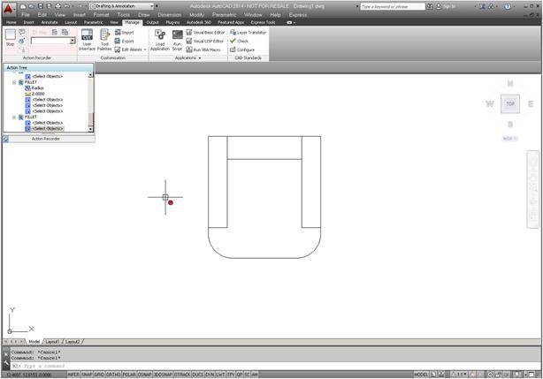
Begin drawing anything you like, such as a piece of furniture, as seen in Figure 15.5. Notice how each action of your mouse, keyboard, menu, Ribbon, and so on is recorded in the log on the upper left.
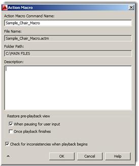
When done, press the Stop button and the Action Macro dialog box appears. Give the macro a descriptive name (no spaces allowed) and press OK, as seen in Figure 15.6.
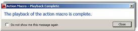
The macro has now been completed and stored as an *.actm file in a default location (which can be changed via Options…→Files). You can put it to use by erasing the chair and pressing the Play button. The macro executes and the chair is drawn. You then see the message shown in Figure 15.7.
This is a very simple example to illustrate the basics. You can get quite complex with macros. For example, you can insert user input or a message. Macros recognize only a few dialog boxes (like layers), so if you need to use one, then make it a command line dialog box via the “- ” (hyphen) prior to typing it in. So, hatch would be –hatch, and so on.
Experiment with this on your own; there are many possibilities.
15.4 Audit and Recover
Although rare, AutoCAD does sometimes lock up and crash (usually a PC hardware or memory issue but can also be software related). In the event of a crash, the drawing is automatically saved but may be corrupted when you try to open it up again. Sometimes, drawings just cause AutoCAD to behave oddly for no specific reason (i.e., commands do not work as expected or just fail). In either case, the drawing needs to be audited or recovered.
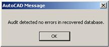
Auditing is the lower-level check. AutoCAD evaluates the integrity of the drawing and corrects some errors. You simply type in audit and press Enter; alternatively, use the cascading menus File→Drawing Utility→Audit. There is no toolbar or Ribbon equivalent. AutoCAD asks about fixing any detected errors (say Yes), cycles through drawing entities, and in a few seconds generates a log similar to what you see next (assuming nothing wrong was found or fixed, as seen here):
Of course, if something is found, fixes are reported. Sometimes, however, audit is not enough and you must recover the drawing. This is not as drastic as it sounds. The recover command is powerful and almost always brings the drawing back as a matter of routine. I can count on one hand the number of drawings that were lost forever due to corruption in 16 years of CAD design. And, even in those cases, going to the previous night’s backups restored the drawing, minus a few hours of lost work.
To use this command, open a blank drawing file, type in recover, and press Enter. Alternatively, you can use the cascading menus File→Drawing Utilities→Recover. There is no toolbar or Ribbon equivalent. You are prompted to browse and find the drawing. Once you select it and press Open, recover runs and generates its own log, as seen next. This particular example was also generated with a clean file. If there were items to fix, recover would have shown the actions taken.
Validating objects in the handle table.
Valid objects 755 Invalid objects 0
Following the log, you see the message box shown in Figure 15.8.
If something were indeed wrong (and then fixed), the drawing would have just opened as normal. Immediately save it.
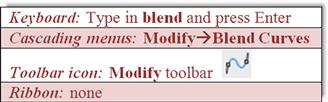
15.5 Blend
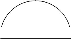
The blend command is a relatively new one; introduced in AutoCAD 2012. It allows you to join, or blend together, linework that is otherwise separate. This linework typically is straight lines or curves, such as arcs or splines. To a lesser extent, some shapes (such as rectangles) can also be blended, although that does not really yield useful results. In all cases, what the blend command does is create a spline between these shapes, curves, or lines. The spline shape can then be modified if needed. To try it out, create two arcs as seen in the top part of Figure 15.9, then follow the steps shown next.
Step 1. Start up the blend command via any of the preceding methods.
![]() AutoCAD says: Continuity=TangentSelect first object or [CONtinuity]:
AutoCAD says: Continuity=TangentSelect first object or [CONtinuity]:
Step 2. Pick the first arc, close to where the blend will start.
![]() AutoCAD says: Select second object:
AutoCAD says: Select second object:
Step 3. Pick the second arc, close to where the blend will end. You see a live preview of the new spline just as you are about to click. A new spline then is created to connect the arcs.
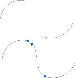
The bottom part of Figure 15.9 shows the results. The new blend has been selected, and the grip points and a down arrow are visible. The down arrow reveals a menu if clicked. This menu lets you choose between showing control vertices or fit points, which presents you with different methods for altering the blend. Experiment with both to see the effects.
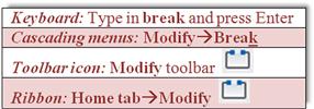
15.6 Break and Join
The break command takes a geometric object and puts a break in it (removes a section, in other words) or, if applied at an intersection with another object, breaks that object at the intersection without actually removing any material. The join command is the exact opposite. It adds material to close the break, but works only in certain circumstances. Let us examine each command closer.
Break, Method 1
To try out the break command, open a new file and draw a line of any size or direction on your screen.
Step 1. Start up the break command via any of the preceding methods. Be sure to turn off OSNAP.
Step 2. Go ahead and click to select the line at some random spot. It turns dashed.
![]() AutoCAD says: Specify second break point or [First point]:
AutoCAD says: Specify second break point or [First point]:
Step 3. Pick another nearby point on the line, and a section between these two points is removed (Figure 15.10).
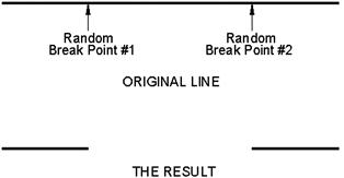
In this method, the first point of the break is somewhat random. When you selected the line, the first point was automatically chosen. However, as shown in the next method, you can select the line to be broken, then, using the First point option, specify exactly where to start the break. We use this to our advantage to create four lines out of two, as seen next.
Break, Method 2
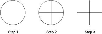
Draw a horizontal line of any size, followed by a perpendicular vertical one that is of equal size. They should cross perfectly in the middle. You have a plus sign. One good trick to do this is to first draw a circle and just connect the four quadrant points with two lines, as seen in Figure 15.11.
Step 1. Start the break command via any of the previous methods.
Step 2. Go ahead and click to select the horizontal line at some random spot. It turns dashed.
![]() AutoCAD says: Specify second break point or [First point]:
AutoCAD says: Specify second break point or [First point]:
Step 3. Type in f for First point.
![]() AutoCAD says: Specify first break point:
AutoCAD says: Specify first break point:
Step 4. Using OSNAPs, select the midpoint of the horizontal line.
![]() AutoCAD says: Specify second break point:
AutoCAD says: Specify second break point:
Step 5. Once again, using OSNAPs, select the same midpoint of the line.
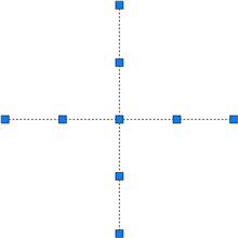
Now, repeat these steps with the vertical line. The result is four lines where there were only two just moments earlier, as seen in Figure 15.12, when the grips are revealed. All four are broken at their intersection.
Join
The join command is included in this discussion because it is the exact opposite of break. It closes the gap between coplanar lines. Note the important disclaimer, however. The join command does not unite lines that are not on the same plane. This means that, if they are not pointing in the exact same direction and are not actually one after the other, then it does not work. To try this out this command, draw two coplanar lines (or use break to put a gap in), as seen in Figure 15.13. Note that join works on an unlimited number of coplanar lines; we are using only two in this example for simplicity.
Step 1. Start the join command via any of the preceding methods.
![]() AutoCAD says: Select source object:
AutoCAD says: Select source object:
Step 2. Select the first line.
![]() AutoCAD says: Select lines to join to source:
AutoCAD says: Select lines to join to source:
Step 3. Select the second line.
![]() AutoCAD says: Select lines to join to source:
AutoCAD says: Select lines to join to source:
A solid line takes the place of the two segments.
15.7 CAD Standards
This is a rather obscure procedure that may be valuable to a few organizations, and I have on occasion recommended it to prime contractors who often find their design files bouncing around from subcontractor to subcontractor. After all the respective additions to the drawings are finished, they are sent back to the main contractor. There, it is found that the standards have deteriorated, as everyone did his or her own thing in regard to layers and text or dim styles. A way to identify and clean up the mess would be useful, hence, the existence of this tool.
The CAD Standards procedures can be a bit confusing, and the process is not effortless nor does it guarantee perfect results. Depending on the damage, you may still need to do manual cleanup of layer properties, errant fonts, and the like. The best defense is to hold all others who may work on your drawings to a high standard from the start and outline what is acceptable and what is not. Obviously this can be challenging in just one office, never mind implementing it for designers at other, remote locations.
Here is the basic idea. Come up with one file that is in great shape. This can be a regular job that is singled out for its perfect or near perfect use of company standards and is of the highest quality and integrity. Then, do a Save As for this job under a .dws (drawing standards) extension. This is your standards file. All others are compared to it as they come in from subcontractors or just other designers.
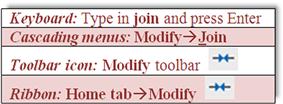
To implement the standards, open up a job that just came in and is of questionable CAD quality. Type in standards and press Enter; alternatively use the cascading menu Tools→CAD Standards→Check…. There is no toolbar or Ribbon equivalent. The Configure Standards dialog box appears, as seen in Figure 15.14.
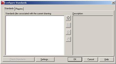
Next use the plus (+) sign to open up the saved .dws file. The file appears in the window on the left with some descriptions on the right. The Check Standards button (lower left) also lights up, at which point you press it to execute the check. The Check Standards dialog box appears, as seen in Figure 15.15.
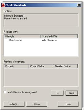
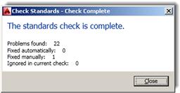
Next, you need to run through the fixes, item by item. Continue pressing the Fix button as AutoCAD runs through the fixes and matches up text, layers, and other items. When done, the Check Complete notice shown in Figure 15.16 displays. In this particular example, four problems were found but none fixed.
15.8 Calculator
The calculator is a surprisingly powerful and versatile tool within AutoCAD, and one that is often overlooked by users. The function’s power and versatility should come as no surprise, as AutoCAD itself is highly mathematical software, a calculator in itself, performing complex operations “under the hood” as you draw, copy, and rotate objects.
The calculator function can perform all regular and scientific calculations you would expect from a handheld device; in addition, it can assist you in the construction of geometry and even allows you to use AutoLISP, a programming language. A full description of the calculator command can take up dozens of pages, so we explore only the basics here. However, we take a look at one example of construction assistance using the transparent line command cal and one example of the actual graphic calculator tool (QuickCalc) to do unit conversions. You are encouraged to read the Help files for a wealth of additional information.
First, a brief overview of the basic cal command. This was the original version of the calculator. It is a command line tool enabled by typing in cal and pressing Enter. AutoCAD then says: >>Expression:, at which point you can enter some math function using the familiar characters such as +, –, *, and /. Pressing Enter again yields an answer.
Not too long ago the limit of the calculator was+32,767 and−32,768 as the largest displayable final integer, but that restriction was lifted somewhere around the AutoCAD 2005 release, and you can now work with integer numbers between+2,147,483,647 and−2,147,483,648 (that is 2 to the 15th and 31st powers, respectively, if you really wanted to know where those seemingly random numbers came from).
Let us use the previously described cal command to assist in design, because crunching numbers alone can be done by your handheld or Windows calculator. Suppose you need to offset a line one half of some number, but you do not know what that value is (say, one half of 17.625). Instead of reaching for that calculator, let AutoCAD do both: calculate one half of 17.625 as well as offset the line, all in one command. To do this,
1. Draw a line of any reasonable size.
2. Start the offset command via any method.
3. You do not know the offset distance so let us use the calculator.
4. Type in ’cal (the apostrophe makes cal, or any command, temporarily transparent, meaning you can enter it without exiting out of another, in-progress command, which in this case is offset). Press Enter.
5. The >>>>Expression: prompt asks for the expression. Enter 17.625/2 and press Enter.
6. Your answer (8.8125) appears, and you may resume the offset command.
7. Continuing as usual, select the line and pick a direction to complete the offset and Esc to exit.
This was a very simple case of how the calculator assists in design tasks. It can do a lot more in that regard and you are encouraged to examine the Help files for additional examples.
The calculator function is not just a typed command line but also now comes in a graphic version. If you use this graphic version, you are using what is referred to as a QuickCalc. It is almost a whole new command all to itself and has quite a bit more functionality.

Start up the QuickCalc command via any of the preceding methods and you see Figure 15.17.
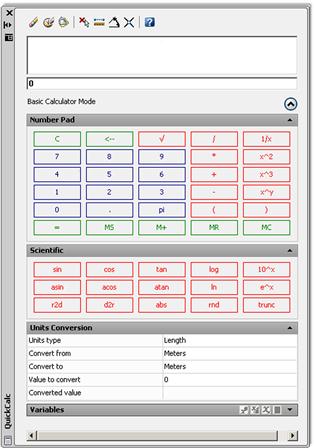
The Number Pad and Scientific keypads are self-explanatory. If you ever used a handheld calculator, you should be right at home with this one. Variables, at the bottom, are not covered, but Units Conversion deserves a special mention. It is a very useful tool for converting between a wide variety of Length, Area, Volume, and Angular values. Simply select from the fields on the right (drop-down arrows appear) and enter the values to convert just below that. A converted value appears according to what you requested.
15.9 Defpoints
Defpoints is not a command, but rather a concept that appears often and bears a short mention. Defpoints stands for definition points, and they appear in the drawing (and mysteriously in the Layers dialog box, where most users first notice them) as soon as you add any dimension to your drawing. What are they exactly? They are the tiny points where a dimension attaches itself to the object being dimensioned. The Defpoints layer does not go away easily and usually prompts questions from students as to its nature and intent. The layer fortunately does not plot, and you can pretty much disregard its existence if you choose. One benefit of it not plotting is that you can put any objects that you do not want to see on paper on it (such as viewports, as is discussed in Chapter 10). In fact, that is exactly what many users do, though a dedicated VP layer is recommended instead. In conclusion, do not worry about Defpoints and continue on.
15.10 Divide and Point Style
Divide does exactly what it advertises; it divides an object into equally spaced intervals. Note, however, that the object is not actually broken into those segments (that is for a break command to do) but rather just divided by equally spaced points. Then, you can use these points as guides for further work. Let us give this a try.
Step 1. Draw a horizontal line of any size.
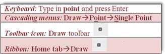
Step 2. Type in divide and press Enter. Alternatively, you can use the cascading menu Draw→Point→Divide. There is no toolbar or Ribbon equivalent.
![]() AutoCAD says: Select object to divide:
AutoCAD says: Select object to divide:
The line looks the same, with no apparent divisions. It seems as though the command has not worked. It actually worked just fine, and the line is divided into the ten segments using nine points, as expected. The problem is that you cannot see the points; they are obscured by the line, and we need to change the point style to something more visible. Using the cascading menus, select Format→Point Style.... You then see the dialog box shown in Figure 15.18.
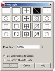
Select a point style that is not too complex; the X format in the top row (second from right) is a popular one. Press OK, and the divided line appears as you were expecting it, divided into the ten visible segments (Figure 15.19).
So, how exactly can you use this to your benefit? Well, the Node OSNAP, which is discussed later in this chapter, allows you to connect to points. If you activate it, you can attach new geometry, perhaps new lines, to those Xs. This is quite useful in basic construction and layout. Note an interesting quirk. If you zoom in or out, the points change size, but revert back to “standard” size upon typing in regen.
15.11 Donut
Although this command sees only occasional use, it is still worth a mention. It creates exactly what it advertises: a donut of varying size. Broken down into its components, a donut is two circles of different size, one inside the other, and a solid hatch fill. You can technically create this shape with existing techniques, but the donut command just makes it easier. You have control over the sizes of both circles and, as a result, the size of the donut. The inner fill is always a solid hatch. Let us give it a try.
Step 1. Start the donut command by typing in donut and pressing Enter. Alternatively you can use the cascading menus Draw→Donut.
![]() AutoCAD says: Specify inside diameter of donut<0.5000>:
AutoCAD says: Specify inside diameter of donut<0.5000>:
Step 2. You can accept this by pressing Enter or type in another value (we accept the 0.5 in this example).
![]() AutoCAD says: Specify outside diameter of donut<1.0000>:
AutoCAD says: Specify outside diameter of donut<1.0000>:
Step 3. Once again, you can accept this value or type in your own (we accept the 1.0 in this example).
![]() AutoCAD says: Specify center of donut or<exit>:
AutoCAD says: Specify center of donut or<exit>:
Step 4. Click anywhere on the screen and the donut appears, as seen in Figure 15.20.

15.12 Draw Order
Draw Order refers to the stacking order of objects positioned one on top of another. This feature is commonly used in most graphic design programs and has an occasional use in AutoCAD as well. The stacking order is usually not of major concern in day-to-day basic drafting. If items intersect, the one drawn last is on top; and in cases of two intersecting lines, the intersection point is 1 pixel in size, hardly worth a second thought.
Sometimes, however, such as when two or more hatch patterns are stacked, the order is critical. We use this feature later in this chapter to great effect when we discuss Wipeout. For now, just know where the Draw Order command is. It is found in the cascading menu under Tools→Draw Order, with options for Objects, Text, Hatches, and Dimensions.
Bring to Front and Send to Back send objects strictly to and from the top and bottom of the order, while Bring Above Objects and Bring Below Objects are more selective, moving items one step at a time. With these four tools, you can arrange any amount of objects in any order.
15.13 eTransmit
The purpose of this command is to assist with emailing drawings. The problem is that, when drawings are sent out, items can be inadvertently omitted. These omissions may include something major, like associated xrefs, or something secondary, such as fonts and styles. As a project grows more complex it is easy to forget to send xrefs and even easier to forget about the unique fonts, styles, and .ctb files that have been generated over time. The recipient of the email may have only some of these and what he or she downloads and reconstructs on that end may not be quite what you may have intended to be seen.
The eTransmit command is a go-getter of sorts. It sniffs out every associated file and everything else that may be relevant to recreate the file(s) in a new location as originally intended. Then, it packages everything together in a folder and sends it out. While veteran users have remarked that an experienced and aware designer needs to always have a clear idea of what to send (eTransmit is a relatively recent addition to AutoCAD after all), it is still a valuable tool for novices and experts alike.
So, what is (and what is not) included in the eTransmit transmittal? Here is a partial list of what is included. You should know of most of these files. If not refer to Appendix C.
*.dwg: Root drawing file and any attached external references.
*.dwf: Design web format files that are attached externally to the root drawing or xrefs.
*.xls: Microsoft Excel spreadsheet files that are linked to data extraction tables.
*.ctb: Color-dependent plot style files used to control the appearance of the objects in the drawings of the transmittal set when plotting.
*.dwt: Drawing template file associated with a sheet set.
*.dws: Drawing standards file associated to a drawing for standards checking.
Here is a partial list of what is not included. Do not worry if you do not recognize all these formats. You will know most of them by the end of Level 2.
*.arx, *.dbx, *.lsp, *.vlx, *.dvb, *.dll: Custom application files (ObjectARX, ObjectDBX, AutoLISP, Visual LISP, VBA, and .NET).
To use eTransmit, save your work but keep the file open. Type in etransmit and press Enter. Alternatively you can use the cascading menu File→eTransmit…. There is no toolbar or Ribbon alternative. You are asked to save the file if it has not been saved yet. Then, the dialog box in Figure 15.21 appears.
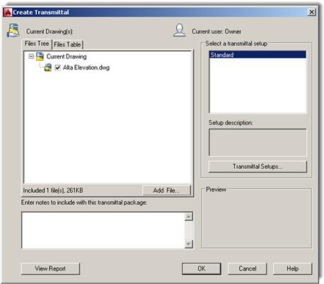
The procedure is highly automated, but you do have to select a few parameters. The current drawing that is open is the one that is packaged together. Some of the included items are shown in the file tree. Expanding the+signs shows specific files (which you can deselect if desired). You also can add more drawings to the transmittal using the Add File… button. If you are fine with just the current drawing (and what is included in it), then press the Transmittal Setups… button. You then see the dialog box shown in Figure 15.22.
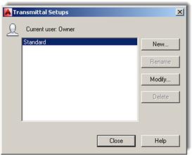
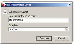
Let us create a new setup as an exercise. Press the New… button, and the dialog box in Figure 15.23 appears. Give the transmittal a name and press Continue. The dialog box in Figure 15.24 then appears.
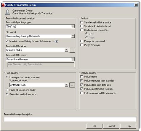
All you really have to do here is visually check all the settings. Looking at the fields from the left, top to bottom, we see the Zip option for actually sending the files (recommended), followed by a variety of information related to formats, names, and locations. Unless you have a specific reason to change something, leave everything as default. On the right-hand side, top to bottom, leave everything under the Actions category as default (unchecked) as well as everything under the Include options category (middle three boxes checked).
When done press OK, then Close in the next dialog box (Figure 15.22), and finally OK in the main setup box (Figure 15.21). You are asked where to put the Zip file and for any last-minute name changes. Pressing Save drops the Zip file into its place, and it is ready for emailing.
15.14 Filter
Filters were briefly discussed in the context of advanced layers (Chapter 12). While the ideas introduced here are roughly similar, the application is slightly different, so let us review them from the beginning.
Filters are nothing more than a method to isolate and select objects using their features or properties. So, for example, you can isolate and select all the circles by virtue of them being circles, and find green objects because they all have the color green in common. You can also add together properties and create requests like “Find me circles that are red only” and so on. This is a good tool for quickly finding stuff in a complex drawing. Once you find these objects, you can change their properties, delete them, or do whatever else is needed.
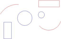
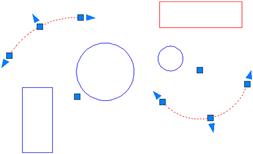
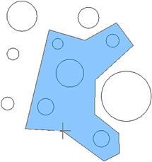
To experiment with filters, let us first create a simple drawing that is just a collection of shapes. Draw the set of circles, rectangles, and arcs seen in Figure 15.25. Then, change the shapes’ colors to blue or red.
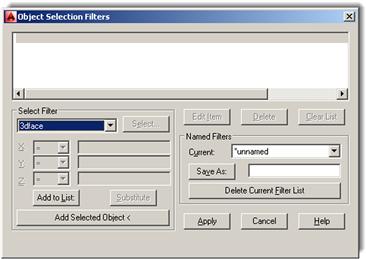
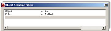
Type in filter and press Enter. There is no cascading menu, toolbar, or Ribbon equivalent. Object Selection Filters appears, as shown in Figure 15.26. The procedure here is to first select the filter, then add it to the list, and finally apply it.
Select Arc from the Select Filter drop-down menu on the left. Then, press the Add to List: button just below that. For good measure, let us also add the color red. Select the color from the same Select Filter menu. Notice, at that point, the Select button lights up. Go ahead and select the color red. Then, press Add to List:. Your filter should look like Figure 15.27.
Now, press the Apply button. AutoCAD asks you to select objects. Select everything by typing in all. Every red arc in the drawing becomes dashed after the first Enter. Press Enter again and the grips come on, as seen in Figure 15.28. Now type in Erase and press Enter. Because they are selected, all the red arcs disappear. Filters can be saved for future use via the Save As: button and the listing can be modified or deleted via the Edit Item, Delete, and Clear List buttons.
15.15 Hyperlink
The hyperlink command attaches a hyperlink to either an object or text. During this process, you are asked to specify what this hyperlink opens when activated. It can be a website (usually) or a document (sometimes). In either case, it is a great command to quickly access additional useful information. Someone, for example, can see a drawing of a product and follow the link to a website of the manufacturer or call up an Excel file that lists all the specs of a design.
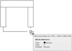
To try out the hyperlink features, draw a symbol for a chair (make a block) and a text website address, as seen in Figure 15.29.
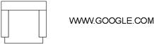
We would like to link the chair (an object) to a furniture website (IKEA®, for example) and link the Google text (a text string) to the Google website.
Type in hyperlink and press Enter. Alternatively, you can use the cascading menu Insert→Hyperlink... There is no toolbar or Ribbon equivalent. AutoCAD asks you to select objects. Go ahead and pick the chair block. The dialog box in Figure 15.30 then appears.
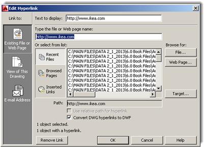
Enter the name of the desired website in the appropriate field. That is where it says: Type the file or Web page name, not Text to display. Not much else needs to be done, so press OK. Repeat the process for the Google text.
Hover your mouse over the chair then the Google text and notice there is something new. A hyperlink symbol appears, with text prompting you to hold down the Ctrl key and click to follow the link (Figure 15.31). If your computer is currently connected to the internet, go ahead and do that in both cases (chair and Google website) to bring up the respective websites.
There is an interesting variation to this, as mentioned earlier. You need not attach a website to the link. You can also attach a regular document, so it is called up when the hyperlink is clicked on, as before. Pretty much anything can be attached if it can be found and the computer can run the application: Word, Excel, PowerPoint documents; pictures; videos—you name it.
To do this, follow the same steps as before, but this time select the File… button under the Browse for: header on the right side of the dialog box. Find the file of interest, double-click on it, and OK the Hyperlink dialog box. That is it; the document is now attached to your object or text and supersedes any other links you may have.
As a final note, recall that Express Tools have a category called Web Tools. We skipped discussing them in Chapter 14 because the hyperlink command was not yet introduced. Take a few minutes now to look over what is available. These express commands include tools to Show, Change, and Find & Replace URLs. These are useful when you have multiple URLs in your drawing and need to manage them. The three tools are very straightforward to use, and we do not spend any further time on them.
15.16 Lengthen
The lengthen command is quite a bit like the extend command in its effect but goes about doing it differently and is worth adding to your AutoCAD vocabulary. The command works by lengthening nonclosed objects, such as lines or arcs (circles and rectangles do not qualify). You can lengthen the objects by change in size [DElta], by percentage added or subtracted [Percent], by total final size [Total], or dynamically “on the fly” [Dynamic]. All this applies to angles (of arcs) as well. To try it out, draw an arc and a line (Figure 15.32).
Step 1. Type in lengthen and press Enter. Alternatively, use the cascading menu Modify→Lengthen. There is no toolbar or Ribbon equivalent.
![]() AutoCAD says: Select an object or [DElta/Percent/Total/DYnamic]:
AutoCAD says: Select an object or [DElta/Percent/Total/DYnamic]:
Step 2. Pick the Percent choice by typing in p and pressing Enter.
![]() AutoCAD says: Enter percentage length<100.0000>:
AutoCAD says: Enter percentage length<100.0000>:
Step 3. Enter a value such as 150 and press Enter.
![]() AutoCAD says: Select an object to change or [Undo]:
AutoCAD says: Select an object to change or [Undo]:
Step 4. Pick the line and it lengthens 150%. Press Esc to exit the command.
The process is essentially the same with the arc and other lengthening options. Repeat the command several times and run through each option.
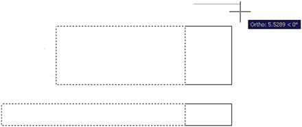
15.17 Object Tracking (Otrack)
Object snap tracking is a drawing aid that allows you to find various OSNAP points of an object and connect to them without actually drawing anything that touches that object, a sort of remote OSNAP. This function can be activated when the OTRACK button is pressed in at the bottom of the AutoCAD screen and is deactivated when the button is pressed back out. The best way to see the purpose and function of this command is to try it. Draw a series of rectangles or squares spaced some distance apart, as shown in Figure 15.33. You need not number them; that is only for identification purposes.
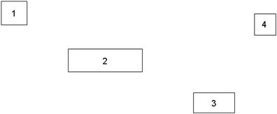
What we want to do is connect a series of lines from (and to) the midpoints of each of these shapes via right angles (not directly). An example of this may be a cable diagram or an electrical schematic. One way would be to start a line from the midpoint of the right side of shape 1, stop somewhere randomly, and repeat the process from the top of shape 2. Then, you can use trim, extend, or fillet to connect the lines. This, however, is cumbersome and slow.
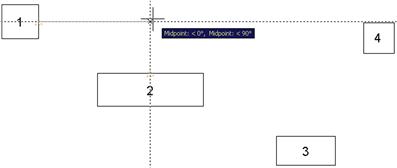
A better way is to begin the line from the right side midpoint of shape 1 as before (turn on ORTHO also) but then activate OTRACK and, without clicking, position the mouse over the midpoint of the top of shape 2. A straight dashed vertical line appears. Follow that dashed line back until the mouse meets the straight horizontal dashed line. Then and only then, click once and continue to draw the line to shape 2. This is shown in Figure 15.34. Notice what OTRACK does. It senses where that midpoint of shape 2 is and gives you a position to confirm and click before proceeding. Complete similar lines from the bottom of shape 2 to the top of shape 3 and then 4.
15.18 Overkill
This interesting command is technically part of the Express Tools under Modify→Delete duplicate objects, but it is more entertaining to type in its rather dramatic other name. What overkill does though is quite useful. It deletes duplicate objects that overlap each other. In the 2D flat world of AutoCAD, it can be quite challenging and time consuming to find these overlaps, especially if similar shapes and colors are involved. With overkill, you simply select the offending objects and AutoCAD figures out which to keep and which to delete, effectively merging them all into one.
To try it out, draw five lines, one on top of another. Although it may not be obvious to a novice, an experienced user notices these lines are a bit darker and “fuzzy,” indicating the presence of an overlap; it is subtle but there. Now type in overkill and press Enter. AutoCAD asks you to select objects. Select all five lines using a Window or Crossing (not one at a time) and press Enter when done. The dialog box in Figure 15.35 appears. Note that if you have seen this command in older versions of AutoCAD, it has been redesigned somewhat.
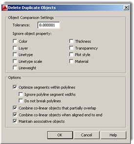
You can leave all the defaults as they are, pressing OK to have all the lines merge into one line. This is probably the simplest application of the overkill command. However, what if the lines are on different layers?
In that case, you have to check off Ignore LAYERS and the command merges the layers into one. Numeric fuzz works by comparing the distances between nearly overlapping objects and acts on them if the distance falls inside the fuzz value. Overkill has other useful features as well, so go through the command, referring to the Express Tools Help files for more information.
15.19 Point and Node
You have already seen and used points when we discussed the divide command earlier in this chapter. In that example, points were created as a means to divide an object. To see them clearly, you needed to modify the form of the point, from a dot to something more visible, using Format→Point Style….
The point command can also be used to create points from scratch, as described next.
Step 1. Start the point command via any of the preceding methods.
![]() AutoCAD says: Current point modes: PDMODE=3 PDSIZE=0.0000Specify a point:
AutoCAD says: Current point modes: PDMODE=3 PDSIZE=0.0000Specify a point:
As you may imagine, points by themselves are not too useful, but change them to an X and they can be used to create “anchors” to which you can attach geometry. For this, you need an OSNAP point that can do that. Called Node, it is one of the 13 OSNAPs. The symbol is a circle with an X superimposed on it. Go ahead and activate Node and practice drawing some lines that originate from the points you just created.
15.20 Publish
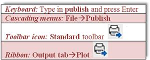
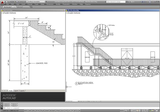
The Publish command is a convenient way to print multiple sheets (layouts) all at once. This command depends on knowing the basics of Paper Space, so you may want to review Chapter 10 if needed. Assuming, however, that you have done so, the idea here is quite simple. When a file with multiple layouts is opened, the Publish command sees them and allows you to print them all at once, as opposed to clicking on each tab one at a time and using the plot command. For this example, a file called Alta Elevation is opened. It features a design spread out over two layouts: a Plan View and an Elevation View. The Publish command is then started via any of the following methods.
The dialog box in Figure 15.36 then appears. Note that it can be expanded, if it is not, by pressing the Show details button on the lower left.
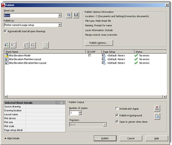
The dialog box features some options to fine-tune publishing, such as adding additional sheets, plot stamp, deciding how many copies, and a few others. All you have to do at this point is just press the Publish button on the bottom, and AutoCAD prints out one copy of every single layout the file contains. It is quick and easy and saves time. Go ahead and explore this very useful command on your own for additional features.
15.21 Raster
Raster is a term you may hear in AutoCAD circles, and it is not so much a command as a concept in graphic design. A raster graphic is nothing more than a bitmap, which in turn is a grid of pixels viewable on any display medium, such as paper or a computer monitor. This method of presenting graphics stands in marked contrast to vector graphics, which are based on underlying mathematical formulas. Vectors can be scaled up or down with no loss of clarity, while bitmaps cannot. So raster images are basically pictures. These can easily be inserted into AutoCAD as covered in a previous chapter.
Raster graphics hold a unique place in AutoCAD history. They were needed to implement a massive worldwide conversion from paper-based, hand-drawn designs to CAD files. When it became obvious that computer-aided design was the future, millions upon millions of hand-drawn documents, spanning decades of design work, were scanned into the computer, became backgrounds, and were patiently redrawn. Government and private industries around the industrial world collectively spent large sums of money and many work hours to transform these archives into viable CAD files for future use. Most of this work was done during a ten-year span (1988–1998), although some of it was started prior and some work is still ongoing. I recall putting in some significant screen time doing these conversions early in my career, and for a new AutoCAD user, this was excellent, if boring, practice: scan, draw, print, check, and repeat.
Raster scanning software can be quite sophisticated. At the time, we used regular large sheet scanners that simply pulled up the graphic on the screen. We then tugged at it until it was the right size (by comparing a drawn line to a scanned known dimension). Later, we acquired more sophisticated software that actually recognized shapes and attempted recreating these pieces of geometry with somewhat mixed results. Any smudges, imperfections, or odd shapes could confuse the system. Noise level (sensitivity) settings were used to control how much was picked up, and it was usually better to set it lower, so you could add what was missing rather than constantly erase accidentally picked up junk. As an AutoCAD user today, you may never need these tools, but it is good to know what they are just in case.
15.22 Revcloud
This is a command that thousands of architects were screaming for. Revision clouds, or revclouds for short, are used to indicate changes on a drawing. You can use an ellipse, rectangle, or circle just as well, but these shapes blend too easily with actual design work, and the unmistakable cloud shape is a better choice. Revclouds were once drawn using arcs, an extremely tedious process. Finally, some program-savvy designers wrote routines to automate the process. Autodesk then jumped on board and revclouds were born. Let us give it a try.
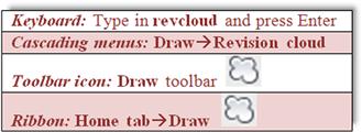
Step 1. Start up the revcloud command via any of the preceding methods.
Minimum arc length: 0.5000 Maximum arc length: 0.5000 Style: Normal
Specify start point or [Arc length/Object/Style]<Object>:
![]() AutoCAD says: Guide crosshairs along cloud path…
AutoCAD says: Guide crosshairs along cloud path…
Step 3. Draw a circular shaped revcloud connecting the last arc to the first one (no extra clicking needed).
Your result should look somewhat similar to Figure 15.37 (you may have to zoom in or out to see the revcloud).

The command has several options. For example, if you do not connect the last arc to the first and instead just right-click, AutoCAD asks you: Reverse direction [Yes/No]<No>:. Here you can actually turn the revcloud “inside out,” though this is rarely done. You can also change the size of the cloud’s arcs by selecting the Arc length option, and even turn objects (like circle and rectangles) into revclouds using the Object option. Take the time to experiment with all of these.
15.23 Sheet Sets
Like many new features in AutoCAD, these are not revolutions but rather evolutions of previous ideas. This tool, introduced in AutoCAD 2005, was meant to combine some aspects of Paper Space layouts and the Publish command with a few new twists, to create an “all under one roof” method of setting up the presentation and printing of a project. The idea is to set up sheet sets (1 Layout=1 Sheet) that define exactly what is needed to plot the entire job correctly. These sheets can come from different drawings and even different jobs and are grouped together by their respective categories. The idea is that they are now easier to handle and organize.
The industry has shown some reluctance to use a tool that somewhat duplicates existing functionality (even if new features are added), but a few organizations, not surprisingly ones that produce jobs that span dozens of sheets, took to this sheet set idea. We provide a brief overview, and you can decide if you want to pursue this further.
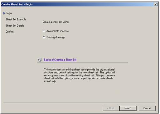
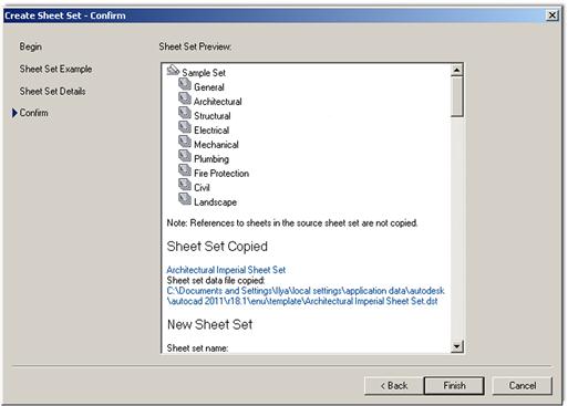
To create a sheet set, you need to set it up. Go to File→New Sheet Set… and you see what is shown in Figure 15.38. Select the first choice, an example sheet set, and press Next>. What is shown in Figure 15.39 appears.
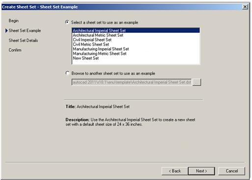
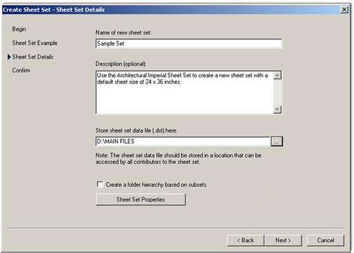
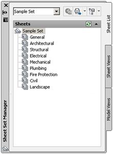
Select the appropriate sheet set, Architectural Imperial for example, and press Next>. Figure 15.40 appears. Here, you can give the set a name and location. Press Next>, and what is shown in Figure 15.41 appears. The various sheet sets, sorted by category, are visible. Press Finish, and the Sheet Set Manager appears, as seen in Figure 15.42.
This was all just to set up the basic sheets (placeholders). They are still blank and need drawings associated with them. Right-click on the Architectural folder and select Import Layouts as Sheet…. What is shown in Figure 15.43 appears.
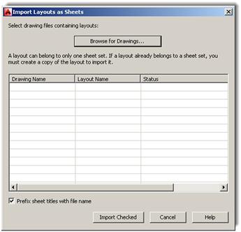
You now have to browse for the right drawing associated with the Architectural layout. Continue down the categories until all are filled. This is just the basic idea of sheets sets. It is an extensive tool that can span many more pages of descriptions, and you should explore some of it on your own.
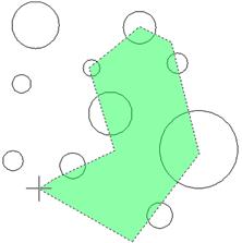
15.24 Selection Methods
What we outline here are a few other methods of selecting items that you may have not yet seen: the fence (F), Window polygon (WP), and Crossing polygon (CP). All these are applicable when selecting objects for a number of operations such as erase, move, copy, and trim.
To try out the Window polygon,
Step 1. Draw a set of circles, as seen in Figure 15.44.
Step 2. Begin the erase command via any method you prefer.
Step 3. When it is time to select objects, type in wp for Window polygon and press Enter.
![]() AutoCAD says: First polygon point:
AutoCAD says: First polygon point:
![]() AutoCAD says: Specify endpoint of line or [Undo]:
AutoCAD says: Specify endpoint of line or [Undo]:
Step 5. Continue to “stitch” your way around the circles you wish to select, and right-click when done.
Notice the difference here between the standard Window selection tool (strictly rectangular in nature) and the flexible “any shape you want it” Window polygon (Figure 15.44). Its action, of course, is similar; everything it encloses is selected.
To try out the Crossing polygon,
Step 1. Draw another set of circles, as seen in Figure 15.45, or just undo your previous steps.
Step 2. Begin the erase command via any method you prefer.
Step 3. When it is time to select objects, type in cp for Crossing polygon and press Enter.
![]() AutoCAD says: First polygon point:
AutoCAD says: First polygon point:
![]() AutoCAD says: Specify endpoint of line or [Undo]:
AutoCAD says: Specify endpoint of line or [Undo]:
Step 5. Continue to “stitch” your way through the circles you wish to select, and right-click when done.
As you can see, the Crossing polygon (Figure 15.45) works the same exact way as the Window polygon, except anything it touches gets selected, much like how the regular Crossing operates.
The fence option works by having a drawn line by the cutting tool during a trim command and selects multiple lines to be trimmed. Draw a bunch of vertical lines, and one horizontal line, as seen in Figure 15.46. Then execute the trim command, but when it is time to select the lines to be trimmed, type in f for fence, and click twice to draw a line across the lines to be trimmed, finally pressing Enter to make them disappear.
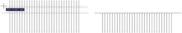
In case you discovered it on your own, yes, you can accomplish the exact same thing using a regular crossing to eliminate the lines once a cutting edge is selected. However, the fence command comes in handy when going around corners, as the flexible line-based approach can bend around any shape, while the rigid rectangular-shaped crossing cannot. Try out both methods, as well as using fence around corners.
15.25 Stretch
This is an easy command to learn and use, and it can work wonders for quick shape modifications. The stretch command uses the Crossing tool to literally stretch shapes. Create two rectangles, as seen in Figure 15.47.
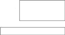
We want to stretch the right sides of both rectangles some distance.
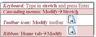
Start the stretch command via any of the preceding methods.
Using a Crossing (this does not work with the Window selector), select the first quarter or so of the rectangles, as seen in Figure 15.48.
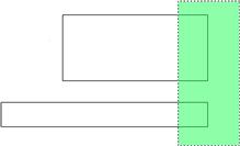
They become dashed. Press Enter and click anywhere to begin stretching them, as seen in Figure 15.49. You need to have Ortho on and all OSNAPs off.
Finally, click elsewhere and the rectangles have a new length. You did not have to explode and redraw them or use grips. You can use the Displacement option to key in specific X, Y, or Z distances or stretch to another OSNAP point. Note that stretch does not work on partially selected circles and it moves, not stretches, fully selected ones.
15.26 System Variables
There is not much to say about system variables except to make you aware of what they are, so if they come up in reading other texts or the AutoCAD Help files, you know with what you are dealing. System variables are Yes/No, On/Off, or 0, 1, 2, 3 types of commands used to indicate a preference or a setting. AutoCAD 2012 has over 850 of them for every conceivable variable (something that changes) in the software, and listing them all is futile, although if you wish to see them all, type in setvar, press Enter, then type in ?, and press Enter twice.
Many system variables are set graphically via a dialog box, and users may not even be aware or know they are changing a system variable. Perusing the Help files and AutoCAD literature, especially on an advanced level, you find many references to them. Knowing system variables is important for those wishing to learn advanced customization (such as AutoLISP).
Here is a useful example that is typed in on the command line. Suppose you are mirroring text and the new set is backwards, as seen in Figure 15.50.
That is not quite right, as you want text to be readable even after mirroring, so some sort of system variable (SV) needs to be set. The responsible SV is called mirrtext, and it is of the On/Off variety represented by 0 and 1. Somehow, it got set to 1, and needs to be 0. Type in mirrtext, press Enter, type in the new value of 0, and press Enter again. Try the mirror command again— it should work fine now.
As mentioned before, this is just one example; there are hundreds of others. Keep an eye out for them. After years of using AutoCAD, you will amass a formidable collection of useful SVs that can resolve some thorny problems for less experienced designers.
15.27 Tables
If you have not yet used tables, here is a quick primer on them. They are pretty much what you might expect, a bunch of rows and columns, with a header on top, ready for you to enter information. You can specify the number of rows and columns and add or take them away at a later time as well. Tables are sort of like low-tech Excel spreadsheets and can be useful in certain situations (like when you need data displayed in a hurry). We cover some basics here and let you explore more on your own.
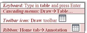
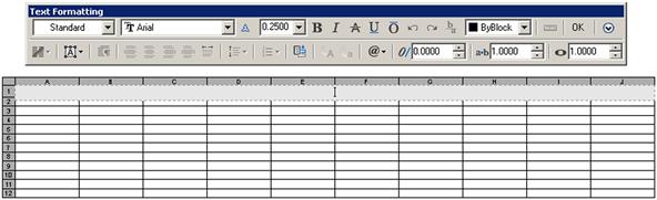
Start the table command via any of the preceding methods. You see Figure 15.51.
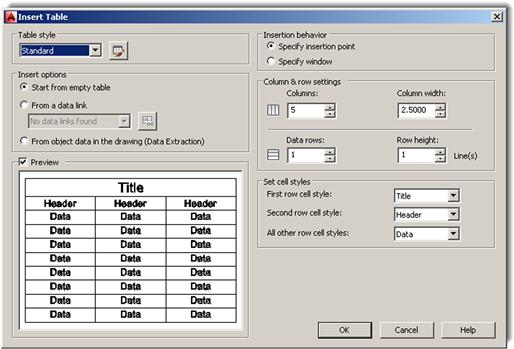
Under the Column & row settings category, set your columns and rows as well as their respective widths and heights (we do a 10×10 here). When done, press OK, and you are asked to click where you want the table to go. When you position it, you see what is shown in Figure 15.52.
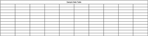
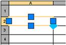
Here, you are asked to set up the header. Type in Sample Data Table and press OK. You see the completed table in Figure 15.53. You can now fill in the table with data by clicking in each cell and typing in values, as seen in Figure 15.54.
There is more to this command, such as sizing and modification of the table, as well as some ability to link up with Excel spreadsheets, so go ahead and explore it further. You can also set up styles of tables by first using the tablestyle command, which gives you the dialog box for “designing” a table (Figure 15.55).
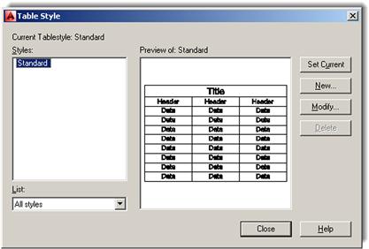
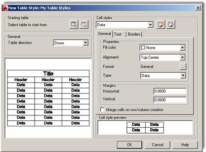
Press New… and give your style a name. You then get the New Table Style dialog box (Figure 15.56). Here you can work with the general properties, text, and borders of the new table, similar to an Excel spreadsheet, and design a custom style that fits your needs.
15.28 Tool Palette
This useful palette, shown in Figure 15.57, can be accessed by typing in toolpalettes, via the cascading menu Tools→Palettes→Tool Palettes, or by pressing Ctrl+3. It may also be on your screen already, but hidden away off to the side. To see it, you have to hover the mouse over the palette’s spine for it to reveal itself. This “autohide” feature can be disabled via a right-click (on the spine) menu, seen in Figure 15.58.
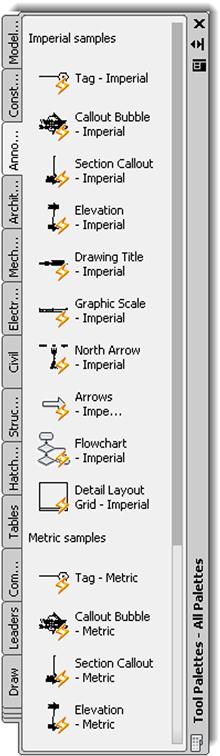
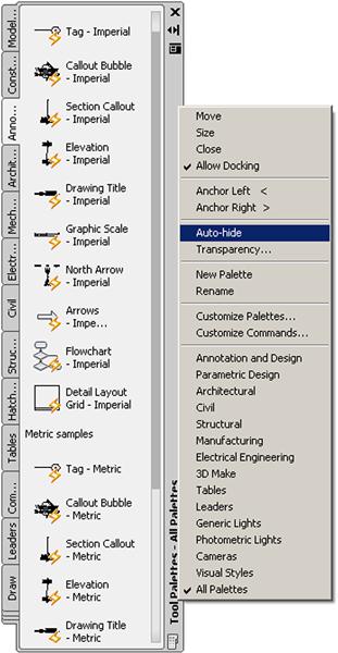
The tool palette represents a collection of commonly used commands and predefined blocks. What you actually see when the palette comes up may be different from Figure 15.57, as it depends completely on what menu is pulled up or what tab is clicked. In all cases, to use this palette, just click on a command (or click and drag), and it is executed as though you typed or selected a toolbar icon. To access more menus, simply right-click on the gray “spine.” As mentioned before, the menu in Figure 15.58 appears.
Even more tabs are available in this palette. Go to the bottom left of the tabs (where it looks like several tabs are bunched together) and left-click. Another extensive menu appears, as shown in Figure 15.59.
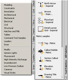
Take the time to go through each of the menu choices. The amount of available blocks is quite extensive.
Although we do not go into this further, you may also customize what tabs you have available by creating your own and adding custom commands and blocks to it. This is similar to creating new toolbars using the CUI, as covered in Chapter 14. You can also modify existing commands in the tabs; finally, the entire palette can be hidden, docked, and even made transparent, so it is always there but you can see what you are doing underneath it, a neat, if distracting, trick. Explore all the options; most are easy to figure out and self-explanatory.
15.29 UCS and Crosshair Rotation
Rotating the crosshairs or the UCS icon is a very useful trick for working with tilted shapes. Not everything you work on will be perfectly horizontal and vertical. Some designs, or parts thereof, will be rotated at some angle; and it would be nice to align the crosshairs to them. This allows for easier drawing and better orientation for the designer. Commands such as Ortho can now be implemented at the new tilted angle.
Rotating the UCS icon is technically not the same as rotating just the crosshairs, but we do not split hairs (so to speak) over the conceptual differences, and we treat both methods as equivalent for now. There are two ways to rotate the Crosshairs/UCS icon: the legacy method prior to AutoCAD 2012 (using snap or the UCS command) and the new method via the UCS icon grips menu, which we cover first.
Method 1
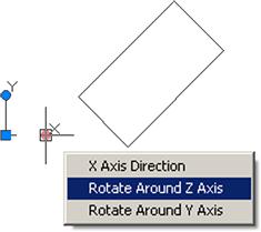
Three releases ago, in AutoCAD 2012, the UCS icon gained some new functionality in the form of grips. It seems like an odd place to add grips—the icon is not a construction object after all—but it works well. To demonstrate, draw a rectangle tilted at a 45° angle and click on the UCS icon. You see three grips appear. The outer ones can be clicked again to manually rotate the icon to any desired angle. The inner one can be used to move the icon around. Each of the grips reveals a menu as well. We ignore the inner grip for now and focus on the outer ones. Select the Rotate Around Z Axis choice (Figure 15.60), and AutoCAD prompts you to enter a rotation angle (also 45° in this case).
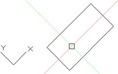
Once you enter the value, the crosshairs rotate and turn a colorful green and red. See the rotation of the crosshairs in Figure 15.61. If you have Ortho on, you can now draw lines that are aligned to your rectangle.
Note that you can achieve the same result by the following steps:
Step 1. Type in ucs and press Enter.
![]() AutoCAD says: Specify origin of UCS or [Face/NAmed/OBject/Previous/View/World/X/Y/Z/ZAxis]<World>:
AutoCAD says: Specify origin of UCS or [Face/NAmed/OBject/Previous/View/World/X/Y/Z/ZAxis]<World>:
Step 2. Type in z and press Enter. You always want to rotate around the Z axis in 2D.
![]() AutoCAD says: Specify rotation angle about Z axis<90>
AutoCAD says: Specify rotation angle about Z axis<90>
Step 3. Type in 45° for this example. The UCS icon is rotated along with the crosshairs.
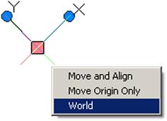
To return back to the usual orientation of the UCS/crosshairs, you can type in ucs, press Enter, and type in w for World, or select World from the center grip menu, as seen in Figure 15.62.
Method 2
This legacy method does something different: It rotates the crosshairs but not the UCS icon. It is a minor variation on the same idea but one of which you should be aware. In 2D AutoCAD, this makes no practical difference, as stated earlier. In 3D, there is a more significant consequence, and the UCS method is used.
Step 1. Type in snap and press Enter.
Step 2. Type in ro and press Enter.
Step 3. For the base point, type in 0,0.
Step 4. For angle of rotation type in per for perpendicular.
To get back to normal, repeat all six steps, except type in 0 at step 4.
15.30 Window Tiling and Tabs
Window Tiling
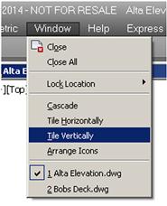
This is just a simple tool for allowing viewing of two drawings side by side in a convenient manner. Open up two drawings in one session of AutoCAD and press Restore Down (middle button) at the upper right for one of the drawings, so the two drawings are tiled one on top of the other. You see something similar to Figure 15.63. Then, select Window→Tile Vertically from the drop-down menu, as seen in Figure 15.64. After the button is clicked on, you see what is shown in Figure 15.65. The active drawing is highlighted.
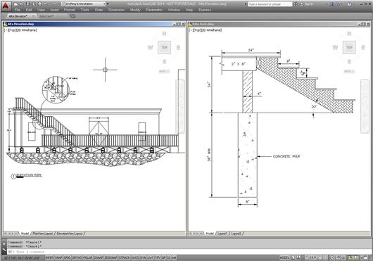
Both drawings are lined up neatly on the screen. You can now click in and out of each and use copy and paste commands to transfer items if necessary. The same thing, of course, can be done for a horizontal tiling.
Tabs
Window tiling is a convenient tool for viewing more than one drawing per screen and you can arrange quite a few side by side. However there is a major down side. Each drawing takes up precious screen space and has to share it with new ones as they come up. Not too bad with two drawing, but the screen gets crowded quickly with three or more.
A more logical approach, which sacrifices the side by side convenience but allows for many drawings to be open and accessed easily, is the tabs tool. These tabs are found at the top of left of the drawing area and look similar to Excel spreadsheet tabs. They are a new feature of AutoCAD 2014, but some third-party vendors have made this available as a customization last year.
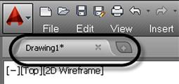
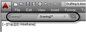
When you first open AutoCAD, there is only one tab (Figure 15.66) representing the primary drawing. If you open other files they appear as new tabs. You can also click on the small plus sign next to the tab to create a new blank file (Figure 15.67). This of course is equivalent to just selecting File→New…. Regardless of how you “collect” these new tabs, you can now cycle through them and work on whichever drawing you need to work on. Each one now takes up the entire screen and need not share the space. It is a good alternative to window tiling.
15.31 Wipeout
For reasons that may not be immediately apparent but are explained in detail, this command is one of the most important in 2D to produce drawings that not only possess extraordinary clarity but are easy to work with and modify. When used properly, wipeout is truly an “insiders’” secret, not known by beginner students, and one of the reasons why drawings done by AutoCAD experts have that intangible “something” that sets them apart from those done by less-experienced designers.
First, let us define what a wipeout is. It is simply a tool that creates a mask (or screen) to block out the viewer’s ability to see other drawn geometry covered by the wipeout. To use it, draw a shape of some sort. Then type in wipeout, press Enter, and click your way around all or part of the shape. When you press Enter or right-click, the shape disappears behind the wipeout, as seen in Figure 15.68.
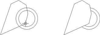
Notice the wipeout itself is still visible (something to be addressed later), but the double circle shape has been partially blocked as expected. Practice using this command a few times just to become familiar with it.
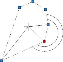
Remember that a wipeout itself is an object. It can be moved, erased, copied, rotated, scaled, and just about anything else you can do to a regular geometric object. You can also click on the wipeout (click on the lines, not the blank center) to activate its grips. Then, the grips can be used to reshape it into any shape whatsoever, as seen in Figure 15.69.
So, what is so important about wipeout? Well, this command allows us to do something very special in 2D work. We can give our designs depth.
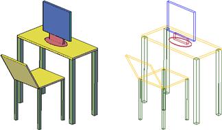
When you look around you in the real world, objects are generally not transparent. So, if you are looking at a bus in front of a building, part of the building is obscured by the bus. If another car were to park between you and the bus, it would obscure part of the bus, and so forth. In 3D, this is no problem at all. All objects are solid, and while they can be viewed in transparent wireframe form, a click of the button gives you rendered models that create an instant illusion of depth. This is important, as it matches our everyday experience and we quickly identify what we are looking at. In the image in Figure 15.70, the chair and the computer monitor both block a part of the computer desk. It is easy to tell what is in front of what in the rendered image on the left, but not as easy with the wireframe image on the right.
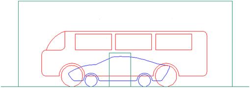
Let us try the same thing with the bus and car, as seen in Figure 15.71. Which is in front of which? You really cannot tell without shading the image, as in Figure 15.72.
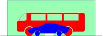
In 2D, though, we have a problem: We cannot shade in the conventional sense. Everything is drawn using lines and nothing is solid, even though it may be in real life. In a plan view of an architectural floor plan, this is not an issue, as we are looking straight down, but what about in elevation view, such as the previous images? A section through a room in elevation view may feature furniture obscuring walls and walls obscuring other items behind them. Or, in electrical engineering, we have equipment on a rack obscuring mounting holes. To provide realism and a sense of depth, we need to somehow obscure our view of items not seen. Of course, you can trim linework behind the object, but what if the object moves? You now have a gaping hole. We need a way to temporarily obscure and hide geometry that is tied directly to the object doing the hiding, so if it moves, the linework reappears. Wipeout is the secret to that trick.
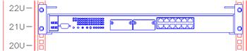
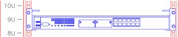
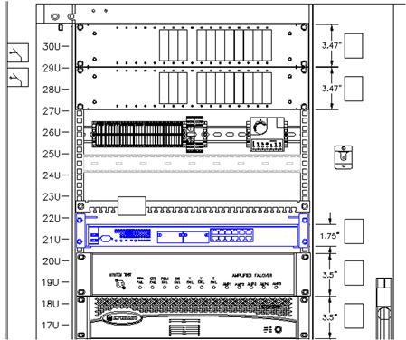
In Figure 15.73, notice how the equipment bolted to the rack obscures part of the rack. Now, if the equipment is moved, such as in Figure 15.74 (notice the numbers to the left change from 20U – 22U to 8U – 10U), the wipeout moves with it and it acts like a solid object. The move is successfully done with no trimming necessary.
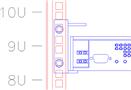
What if you did not have a wipeout? Such is the case in Figure 15.75. Notice that the rack is visible underneath the equipment, giving no indication of depth. You would have to trim lines to achieve this.
In summary, when a wipeout is attached to an object, it prevents anything behind it from being seen, exactly as in real life. So, a bookshelf with a wipeout attached blocks the wall behind it and electrical equipment blocks the mounting holes to which it is attached. Move the object and the wipeout moves, also blocking out whatever you happen to be blocking. This is the technique that the pros use to give drawings a uniquely realistic look in 2D design, and you should learn this as well. Let us go through some details.
The essential steps of making this technique work include the following:
Step 1. Create the drawing of what you are designing, such as the equipment rack in Figure 15.76.
Step 2. Using wipeout, click to trace the outline of the drawing point by point (just the four corners in this case).
Step 3. Using Tools→Draw Order→Send to Back, put the wipeout behind the design.
The object is now “solidified” and can be placed in front of other objects. If you create more objects in this manner, you can simply use the Draw Order tool to shuffle them around top to bottom as needed (as long as all of them are blocks). In this manner, you can create a rather impressive sense of depth and clarity to an otherwise busy drawing.
Take a close look at Figure 15.77. It is a larger section of the same cabinet shown in the previous figures. It could not have been done this way without extensive use of the wipeout command. Notice how it is easy to tell which equipment is in front and which is behind the rack. There are, in fact, several layers of objects: the equipment bolted to the front of the rack, then the rack itself, then the equipment in the back of the rack.
The final item to mention with wipeouts is that they themselves can be hidden (while their ability to hide objects remains in effect). To do this, simply type in wipeout, press Enter, and select f for Frames in the submenu. AutoCAD then says: Enter mode [ON/OFF]<ON>:. If you type in off, AutoCAD turns off all wipeouts on the screen, while preserving their effects on other objects.
15.32 Level 2 Drawing Project (5 of 10): Architectural Floor Plan
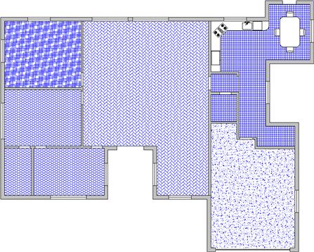
For Part 5 of the drawing project, you add in carpeting and flooring to your floor plan. This is somewhat arbitrary and may or may not be the type of carpeting, tile, or flooring an architect would select on another design. You may use a different pattern, of course, if you wish. As always, be sure to use the proper layering.
Step 1. At a minimum, use the following layer convention:
Step 2. Freeze all layers that are not relevant to the carpeting, leaving only walls, wall hatch, appliances, and windows. Draw a set of temporary lines to block off doorways so the hatch does not bleed from one room into another. Finally, create the carpeting/flooring plan shown in Figure 15.78.
Summary
You should understand and know how to use the following concepts and commands before moving on to Chapter 16:
Exercises
1. Draw the following two rectangles according to the dimensions given. Pedit the width to 0.25" and shade each separately with a solid hatch, color 9. Then, use align to place the 10" box on top of the 4" box. (Difficulty level: Easy; Time to completion:<5 minutes.)
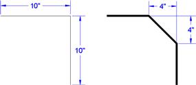
2. Draw the following set of lines and chamfer them to the dimensions shown. Then, pedit the result to a thickness of 0.25". (Difficulty level: Easy; Time to completion:<5 minutes.)
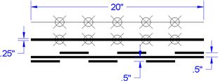
3. Draw the following line and divide it into seven sections using six points of the style shown. Then, pedit the line to a thickness of 0.25" and break it using the break command (First point option) at each of the points. Finally, offset each alternate section 0.5" up and 0.5" down, as shown. (Difficulty level: Easy; Time to completion:<5 minutes.)
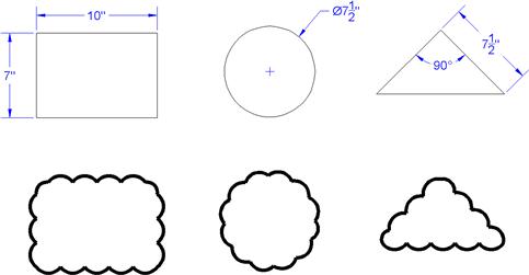
4. Draw the following rectangle, circle, and triangle according to the dimensions shown. Then, use revcloud and the object option to turn each into a revcloud. Finally, pedit the new shapes to a thickness of 0.25". (Difficulty level: Easy; Time to completion: 5 minutes.)