3D Basics
Learning Objectives
In this chapter, we introduce the basics of 3D theory and operating in 3D space. Specific topics include the following:
![]() 3D Workspace: Ribbon, toolbars, and options
3D Workspace: Ribbon, toolbars, and options
By the end of the chapter, you will understand basic 3D theory and be able to navigate in and out of 3D, navigate inside 3D, as well extrude, hide, and shade your designs.
Estimated time for completion of chapter: 1.5 hours.
21.1 Axes, Planes, and Faces
So, what exactly does drawing in 3D mean? It is the ability to give depth to objects, or to expand them into the “third dimension” from a flat plane. This concept should be intuitively obvious—after all, we live in a 3D world. Everything has not just a length and width but also a depth (or height).
It turns out that, as you were learning AutoCAD in Levels 1 and 2, you were in 3D all along. It is just that you did not see or use this vertical third dimension; therefore, everything appeared flat, similar to not seeing the height of a tall building if you are flying directly above it. All this changes as we discuss this hidden dimension and learn how to project into it. For this, we need to start at the very beginning and learn about axes, planes, and faces, because by definition, using the third dimension involves using a third, and previously ignored, Z axis.
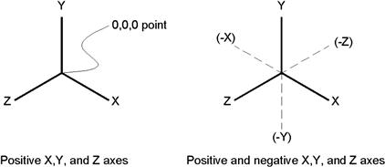
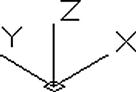
Concept 1. There exists in the Cartesian coordinate system a total of three axes: X, Y, and Z. These axes intersect each other at the 0,0,0 point, as seen in Figure 21.1 (left), and by definition can be positive or negative, as represented by solid and dashed lines in Figure 21.1 (right).
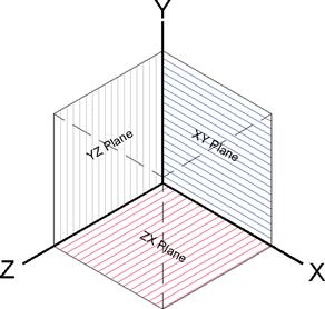
Concept 2. A plane is defined as an intersection of two axes. Therefore, the X, Y, and Z axes can define three unique planes: the XY, YZ, and ZX planes, as seen in Figure 21.2.
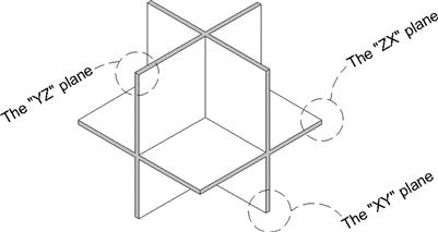
Concept 3. A total of six faces of an imaginary cube can then be formed using the three planes. This can be easily seen if we move the planes out and connect them edge to edge, as in Figure 21.3. For our purposes right now, planes and faces are really the same thing, and we refer only to planes from here on (though the term faces does get some use in related concepts).
The preceding discussion on axes and planes is very important; make sure you completely understand everything thus far. We use both axes and planes shortly.
21.2 3D Workspaces, Ribbon, Toolbars, and 3D Options
Before we can start to work in 3D, we need to set up the appropriate tools, so as to not be distracted with trying to find them later on when we need them. Just as in 2D, you can work in 3D via the Ribbon, toolbars, and the occasional typing. Also, quite a few 3D palettes locate many tools in one spot. You often use a combination of all these tools depending on the situation.
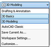
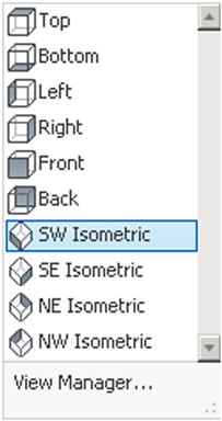
AutoCAD simplifies your work in 3D by allowing you to switch to a 3D workspace. Here you find the Ribbon altered, with many of the needed 3D tools in one place. You have two choices, 3D Basics and 3D Modeling, as seen in Figure 21.4. If you have older versions of AutoCAD installed on your computer, you may see other 3D choices (migrated from AutoCAD 2013, 2012, 2011, etc.), but ignore them and choose 3D Modeling.
You see your AutoCAD screen change to 3D mode. Note the difference in the Ribbon. It now has a full complement of 3D tools available under multiple tabs (Solid, Surface, Mesh, Render, etc.) while retaining some essential 2D tools. Also be sure to restore the menu bar at the top of the screen (see Chapter 1 if you do not recall how). Finally, shut down any toolbars that may have been present, as we bring up some new 3D ones, as described next.
It is very useful to have 3D toolbars on your screen in addition to the Ribbon while you are learning 3D. Despite the overlapping redundancy between the Ribbon and toolbars, a few commands are still found only in the toolbars, so we build a collection of them as we go. If you prefer the Ribbon, you can start eliminating the toolbars after getting acquainted with them as they are introduced.
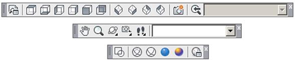
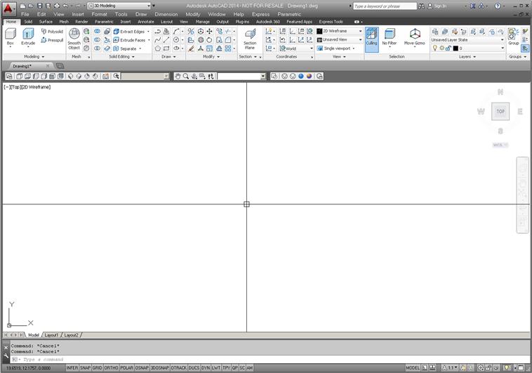
Using Tools→Toolbars→AutoCAD in the cascading menus, bring up the toolbars seen in Figure 21.5. They are View, 3D Navigation, and Visual Styles. Arrange them around the screen area. Your screen should look close to, if not exactly like, Figure 21.6.
It is worth noting that, although you have less and less typing to do in 3D, a few commands are still available only via this method. Also, do not forget, you still have the cascading menus with full 3D tools as an alternative to all of these, in many cases. This covers all four primary methods of interacting with AutoCAD in 3D. As you can see, except for more of an emphasis on graphical inputs (Ribbon and toolbars), the methods remain the same as in 2D.
A few words about 3D and the Options dialog box, first examined in Chapter 14. It is highly recommended that your crosshairs are size 100 (all the way across) in 3D, as this helps a lot with visualizing what you are doing and where in 3D space you are. As a reminder, you can change this under the Display tab. Just as important, you need your UCS icon. In 2D, you may have been tempted to turn it off (it was one of the tips early in Level 1), but here you need it to know where you are in 3D space, and you really cannot work without it. Finally, let us take a look at the 3D Modeling tab under the Options… command that we skipped over in Chapter 14. It is shown in Figure 21.7.
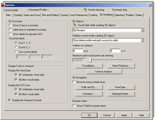
For now, the only suggestion is to make sure the “Show Z axis in crosshairs” option is unchecked (it may already be). It is found all the way at the top left. The 3D concepts are generally much clearer when only two axes are present in the crosshairs. We return to this Options dialog box later in our 3D studies to tweak a few more settings; mostly those at the bottom right (Walk and Fly, ViewCube, etc.). Click on OK and let us jump right into 3D in the next section.
21.3 Entering and Exiting 3D
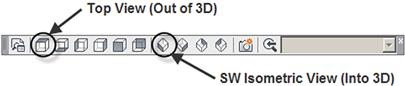
The key to starting out learning 3D is to get into 3D mode and reveal the third axis. The gateway to entering 3D is any of the isometric views, though we use the SW Isometric View most often. The way to exit 3D is any of the flat views (front, back, left, right, etc.), although we use the Top View most often. Let us give this a try using the View toolbar, as shown in Figure 21.8.
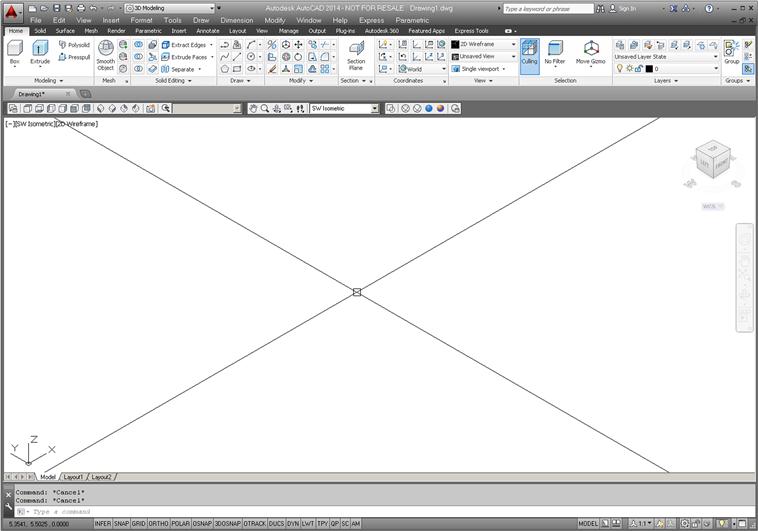
Press the SW Isometric View icon and the screen switches to what you see in Figure 21.9. Examine what happened after going into SW Isometric. The Z axis, previously unseen, is revealed by rotation of the UCS icon and the associated planes. Note how this is reflected in the new position, or shape, of the crosshairs. Note that your UCS icon may be in the center of the screen; we discuss how to get it into the lower left corner in just a moment.
Go ahead and press the Top View icon and go back to 2D. Now that you understand the two essential views, go ahead and press all the other icons to see what view they give you. Icons 2–7 from the left are all 2D views, while icons 8–11 are all 3D. When done, return to the Top 2D view.
Now, try the exact same thing via the Ribbon under the Home tab, View, as seen in Figure 21.10. You have the same basic symbols, so you should know how to proceed.
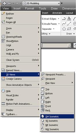
Finally, let us try the same thing via the cascading menu, as seen in Figure 21.11. The path is View→3D Views→SW Isometric (or Top). Once again, the symbols are the same, so you should know how to proceed.
As mentioned just before, when you switch to the SW Isometric View, your UCS icon may stay in the middle of the screen. You generally want it tucked away in the lower left corner (Figure 21.9), just as it was in 2D drafting. To do this, type in ucsicon and press Enter.
Type in n for Noorigin, press Enter, and the icon returns to the corner and does not interfere with viewing design work. In later chapters, we ask it to move out of the corner when we need the icon to be aligned with objects we are working on, but for now this is not necessary, and it just gets in the way.
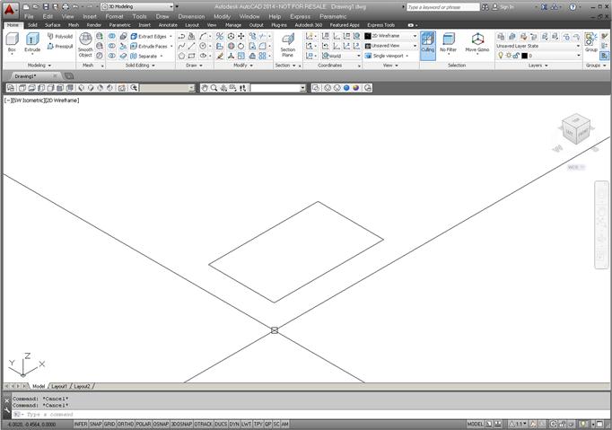
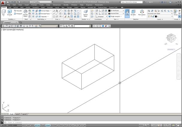
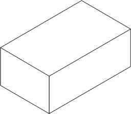
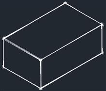
You now know how to get into 3D (SW View) and back to 2D (Top View). So, in 3D, go ahead and draw a rectangle that is 10"×6". You can do this using the rectangle command or individual lines; at this point it does not matter. The result is shown in Figure 21.12.
Here, we come to a roadblock of sorts. Say you would like to draw four sides and a top to create a full 3D box. How do you do this? Although you are in 3D, you have no way yet of actually projecting objects in 3D. This is the subject of the next section.
21.4 Projecting Into 3D
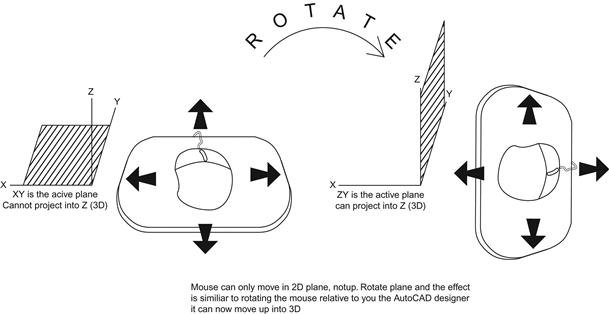
Your input device (universally a mouse these days) is by its nature a 2D device. It works by going forward-back and left-right on your desk or mouse pad but not straight up. This is obviously a bit of a problem for projecting and drawing into the third dimension. Industry software designers and researchers noticed this a long time ago and came up with a simple and elegant solution that was integrated into numerous software packages over the years, including AutoCAD.
When you need to go into 3D, instead of raising your mouse into the air, you simply switch from the “flat” plane you are on to a vertical plane. The effect is immediate; you can now draw “up” relative to you, the observer. To go back to flat, you switch the planes right back. This is shown graphically in Figure 21.13.
You already did this when learning isometric drawing by pressing F5 and cycling through a total of three planes: top, left, and right. We do something similar here in 3D. This is why isometric drawing was important to review. In a way, you already knew some 3D concepts after finishing that chapter.
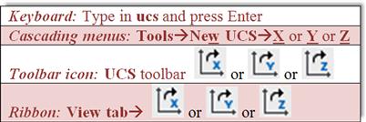
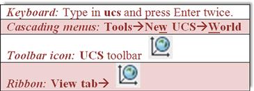
So, how do you actually rotate these planes? Rotating planes is equivalent to rotating the UCS icon. We introduce the various ways you can rotate the UCS icon via the familiar command matrix. You can do this via typing, cascading menus, toolbars, or the Ribbon. If you wish to continue using the toolbars, you need to add the UCS toolbar to your collection (Figure 21.14). We discuss most of this toolbar in Chapter 28, but for now need only three of the icons, as shown next.
To perform the UCS rotation, use any of the methods shown in the preceding command matrix. However there is a slight difference in procedure, depending on what method you choose. Before you start, first read all the way through the steps to get a full understanding!
Step 1(a). If you typed in ucs and pressed Enter, then,
![]() AutoCAD says: Specify origin of UCS or [Face/NAmed/OBject/Previous/View/World /X/Y/Z/ZAxis]<World>:
AutoCAD says: Specify origin of UCS or [Face/NAmed/OBject/Previous/View/World /X/Y/Z/ZAxis]<World>:
Note that the UCS icon will be attached to your mouse. This is not relevant to what we are doing at the moment, and you can ignore it, moving on to choosing an axis in Step 2, then proceeding to Step 3.
Step 1(b). However, if you used the icons, cascading menus, or the Ribbon, then the process of choosing an axis is part of the command right away (as you picked either an X, Y, or Z), and you can skip Step 2.
Step 2. Pick the axis around which you want to rotate: X, Y, or Z.
A very important skill needs to be learned right at the point of Step 1 or Step 2. Around which axis do we need to rotate the UCS icon to be able to draw “up” into the third dimension: X, Y, or Z? It is something you need to be able to quickly identify. Fortunately, in this case, you have a choice of two out of the three axes: either the X or the Y. Rotating around the Z axis does nothing useful (in this example) and just spins the UCS axes around like the blades of a helicopter. Do you see why? So, type in either choice X or Y and press Enter, or if using the other methods, choose X or Y right away. This example proceeds with the X axis being chosen.
Step 3 After the X axis is selected,
![]() AutoCAD says: Specify rotation angle about X axis<90>:
AutoCAD says: Specify rotation angle about X axis<90>:
Step 4 You can just press Enter, as 90° (the default) is exactly what we need.
You should see what is shown in Figure 21.15. The X axis is the “hinge” around which we pivoted and the crosshairs now point in the direction we need to go, which is straight up, relative to you.
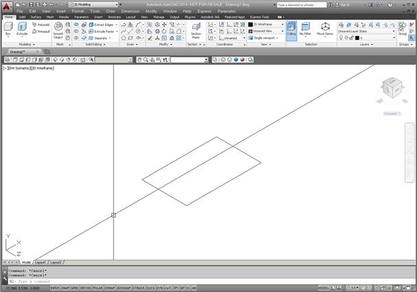
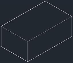
Now, go ahead; using standard drafting techniques, draw a straight line starting from one of the rectangle’s corners and continuing up to any reasonable distance away (using Ortho and OSNAP points, of course). Copy it to the other three corners and copy the bottom four lines (or rectangle) to the top, thereby creating a box. You should have what is shown in Figure 21.16. Note that you may have to use grips to “trim” or “extend” the lines if necessary to create a neatly drawn box.
To bring your UCS icon back to the previous familiar state, as originally seen (and shown again in Figure 21.17) you can do any of the following:
This is called restoring the icon to World View. Practice rotating the UCS icon around all three axes. Notice how the axes act as “hinges” for rotations. You need to recognize which hinge to rotate around later on as we do actual object rotations.
Next, we need to learn some 3D dynamic viewing options, such as Orbit.
21.5 3D Dynamic Views
In 3D, you need to constantly spin the object around to get a good look at it from all sides. AutoCAD has powerful 3D Orbit tools to easily look at your design in real time as opposed to just preset views. Remember that, even though we say that we are rotating the object, really we are not, but rather rotating our view of it.
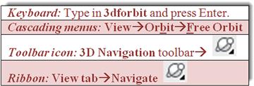
The 3D orbit command comes in several flavors. The “3dorbit” version is constrained to vertical and horizontal movements, while the “3dforbit” (the f stands for “free”), allows for unrestricted movement and will be the version we focus on. There is also the “3dcorbit” (the c stands for “continuous”), which rotates the view nonstop until you exit the command. This is more entertaining than useful but does look impressive in a presentation. You can find all of these cascading down from the 3D Navigation toolbar, so feel free to explore them on your own. We next further describe 3D free orbit. To begin the 3D free orbit, use any of the following methods.
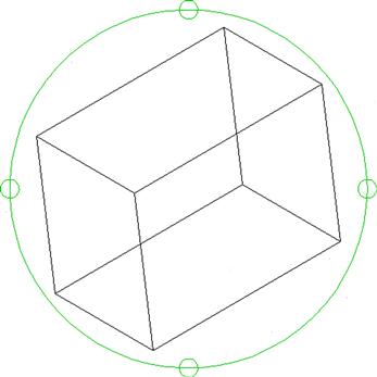
As soon as you click on the Free Orbit icon, a green circle appears, and you are able to do the orbit by clicking down, holding the left mouse button, and moving the mouse around as seen in Figure 21.18. When done just press Esc, and the new view is permanent. To restore the familiar SW view, just press that icon.
What we have done thus far is create a wireframe model. This is a common term in computer-aided design (not just AutoCAD) and simply means the model is not shaded or rendered and resembles a wire that has been shaped into something (a frame), hence, wireframe.
Although we introduced a lot of useful concepts thus far, such as axes, planes, 3D views, 3D orbit, and UCS rotation, the wireframes we created cannot be shaded, as they are essentially “hollow” pieces and contain no surfaces. Creating real solids is the subject of the next section, so go ahead and erase the box; we will create it again.
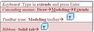
21.6 Extrude
Extrusion is the method most often used to quickly and easily create solid objects and, as such, is perhaps one of the most important commands in 3D. If you prefer toolbars, you need a new toolbar, Modeling (Figure 21.19), to access the extrude command via that method.
We begin the same way as before, by drawing a 10"×6" rectangle, but this time use only the rectangle command, not individual lines, then proceed as described next:
Step 1. Start the extrude command via any of the preceding methods.
Current wire frame density: ISOLINES=4, Closed profiles creation mode=Solid
Select objects to extrude or [MOde]:_MO Closed profiles creation mode [SOlid/SUrface]<Solid>:_SO
Select objects to extrude or [MOde]:
Step 2. Pick the rectangle (AutoCAD will tell you 1 found) and press Enter.
![]() AutoCAD says: Specify height of extrusion or [Direction/Path/Taper angle/Expression]<3.7154>:
AutoCAD says: Specify height of extrusion or [Direction/Path/Taper angle/Expression]<3.7154>:
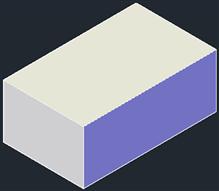
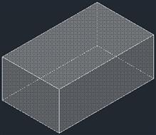
Step 3. You can move your mouse up and down and create a thickness in real time, but it is more practical to type in a value, so go ahead and type in 4 for the thickness. You should see what is shown in Figure 21.20.
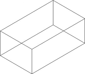
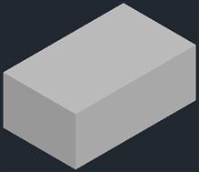
This new, extruded box may at first seem quite similar to the previous one you tried doing. That is because wireframe is not just a method of construction but also a method of presentation. There are some significant differences, however. This box is a real solid model, not just a collection of “wires” spliced together. We can now hide and shade it as described in the next section.
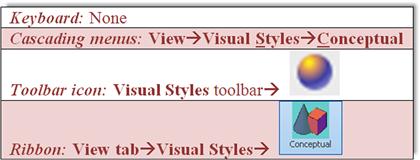
21.7 Visual Styles: Hide and Shade
Visual Styles is an important set of tools that allows you to view your design in a variety of useful ways. We explore two variations of Hide and two distinct versions of Shade: realistic and conceptual. We also look at a few other settings, such as Sketchy and X-Ray.
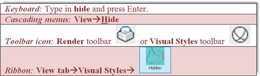
The hide command simply hides wireframe linework that you would not see with a solid object. There are two slightly different variations of it. The first type of hide is temporary while you are viewing a stationary design. The hidden view reverts to wireframe if you try to rotate it or regenerate it. This can be done by simply typing in hide and pressing Enter, via the Hide icon on the Render toolbar (see Figure 21.21), or finally via the cascading menu View→Hide.
The other variety of hide is more permanent and the design can be rotated in 3D while staying fully hidden. That is accomplished via the 3D Hidden Visual Style icon on the Visual Styles toolbar (first shown in Figure 21.6). To return to wireframe, you can no longer just regenerate but must press the 2D Wireframe icon on the same Visual Styles toolbar. All of the previous is summarized in the command matrix shown next. Go ahead and try all the ways to hide your 3D box before moving on.
The result of hiding via the keyboard hide entry, cascading menus, and the Render toolbar’s Hide icon is shown in Figure 21.22. Note how you can no longer zoom and pan. You can still do a Free Orbit, but the hidden lines reappear, so this is useful to just view the design and maybe run off a print.
The result of using the 3D Hidden Visual Style icon as well as the Hidden choice in the Ribbon is shown in Figure 21.23. Note how the background color of the screen changes (which can be changed in the Options…dialog box; Display tab). Also note how you can now zoom and pan. This version of hide is good for continued work on the design while in hidden mode.
Let us now give shading a try. As already mentioned, it comes in two versions, conceptual and realistic. Which you use depends on a variety of shape and background color settings. First, we focus on the default shade, which is the Realistic Visual Style. Start shade via any of the following methods:
The result of this shading is shown in Figure 21.24.
The other style of shade is set as follows. Note that typing in shade is no longer applicable, as that leads to the realistic version of shade being applied by default.
The result of this shading is shown in Figure 21.25.
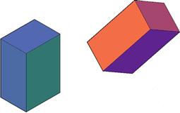
You probably did not notice too much of a difference between the two types of shading. That is because the boxes are not really colored themselves; also, they appeared against the default background, altering the appearance of their own coloring. To appreciate the differences between the two types of shading, observe the two sets of colored and shaded shapes in Figures 21.26 and 21.27.
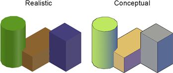
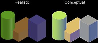
These shapes are set against a white then a black background with the realistic and conceptual shading on and similar colors added to all the shapes. Notice how the softer shading on the right gives a more pleasing picture of the model. For this reason, the Conceptual Visual Style shading is used more often in presenting designs, both on screen and on paper. It is also highly recommended that you set your background to white or black in 3D for a more accurate representation of colors. To return to the unshaded image, press the 2D Wireframe option or icon.
Two more types of presentation views are quickly mentioned: Sketchy and X-ray. Both can be accessed through the Ribbon’s View tab Visual Styles or through the cascading menu’s View→Visual Styles. Try them both out on your box. Figure 21.28 shows the sketchy visual style. It presents a “hand-drawn” rendering of your design and may find some use in a more artistic representation. X-ray makes the shaded shape transparent and is seen in Figure 21.29.
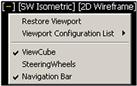
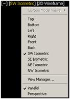
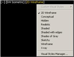
All the views and settings thus far described can be accessed via a set of drop-down menus at the very upper left of the drawing area, shown with a black background for clarity. The first category from the left, [-], is the Viewport Controls. They present various choices for viewports and whether or not to show the ViewCube, SteeringWheels, and Navigation Bar (to be discussed in the next section). The menu is shown in Figure 21.30. Just to the right of that, under [SW Isometric], are the View Controls. They allow yet another way to set and manage the various views. The menu is shown in Figure 21.31. Finally the [2D Wireframe] menu contains the Visual Style Controls. It allows you to set the visual styles, and the menu is shown in Figure 21.32.
After the final discussion regarding the ViewCube, SteeringWheels, and the Navigation Bar in the next section, you should be familiar with almost everything in these menus.
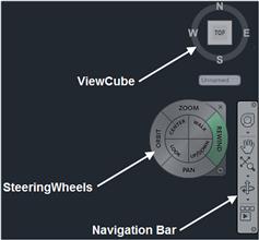
21.8 View Cube and Navigation Bar
You almost certainly have been looking at the ViewCube and Navigation Bar since Chapter 1. The top view of this cube and its friend the Navigation Bar hang out in the upper right corner of your screen and have done so since the beginning, as seen in the 2D top view in Figure 21.33. SteeringWheels (an advanced tool not discussed here) is also seen in Figure 21.33 and is brought up via the first button on the Navigation Bar.
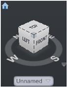
With your box shaded, switch to SW Isometric view. Now that you are in 3D, the bar stays the same, but the cube looks like the one in Figure 21.34.
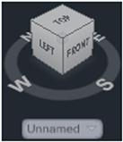
This cube is primarily useful in 3D navigation, and that is why there was no mention of it in the previous 2D chapters. It first appeared in AutoCAD 2009 and is used to dynamically rotate to the graphically shown views, such as top, left, or front. You can click on the faces of the cube, its edges, or its corners; and of course, you can just manually rotate it. Whatever you click on “lights up,” and your design moves accordingly. Additionally, you can press the N, S, E, and W buttons. Go ahead and try it out, returning to the SW Isometric View afterward.
The ViewCube presents no completely new ideas but rather combines a host of various tools in one convenient location. Much of it is equivalent to the toolbar view icons, though you now have the ability to also view a design from a “corner” or an “edge.”
The buttons on the Navigation Bar should also be generally familiar at this point, except for the top button, Full Navigation Wheel, and the bottom button, ShowMotion (also an advanced topic, not covered in this chapter). The rest of the buttons from the top going down are Pan, Zoom Extents, and the various Orbits. Review the functionality of each button.
One last item to mention with the navigation cube is its ability to put you into perspective view. We cover perspective view in later chapters, but you can try it out briefly now. Hover your mouse around the top left area of the cube and a tiny blue house appears, as seen in Figure 21.35.
Click on the house icon and your shaded cube switches to a perspective view (Figure 21.36).
To exit out of this view, right-click on the house and you see the menu in Figure 21.37. Select and click on Parallel and you exit the perspective view.
This is it for the basics. It seems we introduced an endless collection of new concepts, but really it was just six “big ideas,” as listed next:
Review everything carefully; your success in the rest of 3D depends on understanding these basic concepts.
Summary
You should understand and know how to use the following concepts and commands before moving on to Chapter 22:
Exercises
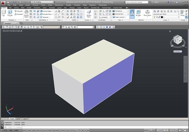
1. In 3D SW Isometric Conceptual Visual Style (CVS), set your units to Architectural and draw a 10’ ×5" rectangle. Extrude this rectangle to 8’ . This is one of several ways to draw a wall. We need this in the coming chapters. Zoom out to extents if necessary and alter the color if you wish. The result is shown next. (Difficulty level: Easy; Time to completion:<3 minutes.)
2. In the 3D SW Isometric CVS, set your units to Architectural and draw a 4" ×3" box. Extrude it to 6" . Now rotate your UCS around the Y axis by 30° and around the X axis by 30°. Then, draw the same rectangle with the same extrusion. Change the colors if you wish. This is what you should get. (Difficulty level: Easy; Time to completion:<5 minutes.)
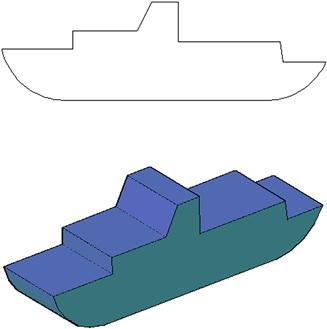
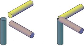
3. In the 3D SW Isometric CVS, set your units to Architectural and draw a 5" circle, extruding it to 25" . Now rotate your UCS around the X axis by 90° and draw the same extruded shape. Then, restore the UCS position, and rotate it around the Y axis by 90°. Draw the same shape again. You should have the three cylinders shown in the left image. Move two of them center to center with the third one as shown in the right image. (Difficulty level: Easy, Time to completion: 5–7 minutes.)
4. In 2D, draw a pline profile of a simple ship as shown next. No exact dimensions are given, and your profile does not have to look exactly like the one shown but somewhat similar. Then, go into 3D SW Isometric and extrude the shape to the approximate depth shown. Color and 3D Orbit to see the shape in its given orientation. (Difficulty level: Easy, Time to completion: 5 minutes.)