
Interest-Point Detection
Beyond Local Scale
Abstract
In this chapter, we propose a novel approach that introduces contextual cues in the detection stage, which is left unexploited in the existing literature. Our motivation is that, so far only local cues are used for detection, which ignores the contextual statistics from neighborhood points. As a result, it is hard to detect the real “interest” points at a higher scale. Furthermore, we also consider the possibility to “feedback” the supervised information to guide the detection stage. In this chapter, we introduce a context-aware semi-local (CASL) feature detector framework to achieve these goals. This framework boosts the interest-point detector from the traditional local scale to a “semi-local” scale, which enables the detection of more meaningful and discriminative features.
2.1 Introduction
In recent years, local interest points, a.k.a., local feature or salient regions, have been widely used in a large variety of computer vision tasks, ranging from object categorization, location recognition, image retrieval, to video analysis and scene reconstruction. Generally speaking, the use of local interest points typically involves two consecutive steps, called the detector and descriptor steps. The detector step involves discovering and locating areas where interest points reside in a given image, e.g., corners and junctions. Such areas should contain strong signal changes in more than one dimension, and can be repetitively identified among images captured with different viewing angles, cameras, lighting conditions, etc. To provide repeatable and discriminative detection, many local feature detectors have been proposed; for instance, Harris-Affine [80], Hessian-Affine [81], MSER [29], and DoG [8].
The descriptor step involves providing a robust characterization of the detected interest points. The goal of this description, in combination with the previous detection operation, is to provide good invariance to variations in scales, rotations, and (partially) affine image transformations. Over the past decade, various representative interest-point descriptors have also been proposed in the literature; for instance, SIFT [9], GLOH [10], shape context [19], RIFT [20], MOP [21], and learning-based (MSR) descriptors [22, 23].
In this chapter, we will skip the basic concepts of how typical detectors and descriptors work. Instead, we discuss in detail a fundamental issue: the detector scale. Generally speaking, the detector operation provides scale invariance to a certain degree, thanks to the scale space theory. However, our concern here is, whether the detection should be at the scale of the “isolated” interest point, or in a higher scope; for example, by investigating the spatial correlation and concurrence among these local interest points. So far, the detector phase of each local feature has been treated in an isolated manner [8, 29, 80, 81]. To this end, each salient region is detected and located separately. We term the proposed detector Context-Aware Semi-Local (CASL) detector.
However, one interesting observation is that, in many computer vision applications, the interest points are proceeded together in the rest recognition or classification steps. In other words, in the rest operations, the recognition or classification system investigates their joint statistics. It is therefore a natural guess that the linking (or middle-level representation) among such “local” interest points would be more important. The inspirations also come from the study of human visual systems [82]. For instance, it has been discovered that the contextual statistics of simple cell responses in the V1 cortex (can be simulated by local filters such as Gabor) are integrated into complex cells in V2 [83] to produce semi-local stimuli in visual representation.
Therefore, it is natural to raise the question: “Can the context of correlative local interest points be integrated to detect more meaningful and discriminative features?”
In this chapter, we explore the “context” issue of local feature detectors, which refers to both spatial and inter-image concurrence statistics of local features. We first review related works on how the local feature context can benefit visual representation and recognition. In general, works in this field can be subdivided into three groups:
• The methods to combine spatial contexts to build local descriptors [19, 85–89]. For example, the shape context idea [19] adopted spatially nearby shape primitives to co-describe local shape features by radial and directive bin division. Lazebnik et al. [87] presented a semi-local affine part description, which used geometric construction and supervised grouping of local affine parts to model 3D objects. Bileschi et al. [89] proposed a contextual description with continuity, symmetry, closure, and repetition to low-level descriptors, with the C1 feature as its basic detector part.
• The methods to combine spatial contexts to refine the recognition classifiers. The most representative work comes from that of Torralba et al. [90–92] in context-aware recognition, aiming to integrate spatial co-occurrence statistics into recognition classifier outputs to co-determine object labels. In addition to these two groups, there are also recent works in context-aware similarity matching [35, 93], which adopts similarities from spatial neighbors to filter out contextually dissimilar patches. It has been shown that by combining the contextual statistics of the local descriptors, the overall discriminability can be largely improved.
• The methods related to biological-inspired models to filter out non-informative regions with limited saliency [94]. Serre et al. [95] presented a biological-inspired model to mirror the mechanisms of V1 and V2 cortices, in which a “S1-C1-S2-C2” framework is proposed to extract features.
The proposed feature detector consists of two steps: First, at a given scale, the correlation among spatially nearby local interest points are modeled, with a Gaussian kernel to build a contextual response. We simulate the Gaussian smoothing and call the output of this step contextual Gaussian estimator. Then, following the difference of Gaussians setting, we derive the difference between nearby scales, which are aggregated into a difference of contextual Gaussians (DoCG) field. We show that the DoCG field can highlight contextually salient regions, as well as discriminate foreground regions from background clutter to reveal visual attention [94, 96]. The proposed “semi-local” detector is built over the peaks in the DoCG field, which is achieved by locating contextual peaks using mean shift search [37]. Each located peak is described with a context-aware semi-local descriptor, which meanwhile ensures the invariance to scales, rotations, and affine transformations.
We further extend our semi-local interest-point detector from the unsupervised case to the supervised case. In the literature, this is related to visual pattern mining [71, 72, 97] or learning-based descriptors [22, 23]. Notably, our work serves as the first one targeted at “learning-based interest-point detection” to the best of our knowledge. This is achieved by integrating category learning into our mean shift search kernels and weights to discover category-aware discriminative features.
This chapter serves as the basis for the entire book about learning-based visual local representation and indexing: First, at the initial local interest-point detection stage, it is beneficial to embed spatial nearest neighbor cues as context to design a better detector, which can serve as a good initial step for the subsequent unsupervised or supervised codebook learning. Second, the learned “semi-local” interest-point detector can be further used in many other application scenarios, to be combined with other related techniques to directly improve retrieval, as will be detailed later in this chapter. For more details and innovations of this chapter, please refer to our publication in ACM Transactions on Intelligent Systems and Technology (2012).
2.2 Difference of Contextual Gaussians
We first introduce how to build the local detector context based on their spatial co-occurrence statistics at multiple scales. General speaking, the “base” detector can be any of the current approaches [81]. As an example, here we use difference of Gaussians [9] as the base detector.
2.2.1 Local Interest-Point Detection
For a target image, we first define the scale space L at scale δ by applying a Gaussian convolution kernel to the intensity component in its HSI color space. As shown in Equation (2.1), I(x,y) stands for the Intensity of pixel (x,y) and G(x,y,δ) is a Gaussian kernel applied to (x,y) with scale parameter δ:
Then, we calculate the difference of Gaussians at the kth scale by subtracting the Gaussian convolutions between the kth scale kδ and the original scale δ (which produce scale spaces L(x,y,kδ) and L(x,y,δ), respectively):
Finally, we identify the local feature candidates as the local maxima within their space and scale neighbors. For a given (x,y) location, there are 3 × 9 − 1 neighbors in total. For each candidate, we construct a Hessian matrix to investigate the ratio between its trace square and determinant. This ratio removes candidates coming from edge points with only signal changes in one dimension. We use the SIFT [9] descriptor to describe each remaining candidate as a 128-dimension local feature vector S. Similarly, other current descriptors [10] can be also adopted.
2.2.2 Accumulating Contextual Gaussian Difference
Then, the distribution of local feature context is quantitatively measured using a proposed difference of contextual Gaussians DoCG field: Our main idea is to estimate the contextual intensity of local features (named contextual Gaussian) based on their spatial distributions with other Gaussian kernel smoothing at different scales. The differences between contextual Gaussian at different scales are then aggregated to produce the DoCG field to quantize the local feature context.
Based upon the above principle, we give detailed formulation as follows: For a given local feature at location (x,y), its contextual Gaussian response is estimated using its neighborhood local feature distributions with Gaussian smoothing at “contextual” scale δcontext:
where SCL(x,y,δcontext) is the estimated contextual Gaussian density at location (x,y) with contextual scale δcontext; i = 1 to n represents the n local features falling within δcontext of (x,y); and Si is the feature vector of the ith neighborhood local feature descriptor.
We then calculate the difference of contextual Gaussians (SDoCG) at the kth scale (kδcontext) by subtracting SCL(x,y,kδcontext) and SCL(x,y,δcontext) between the kδcontext and the δcontext contextual scales:
Note that the above operation differs from the traditional DoG operation [8] which seeks the neighborhood local peaks within the consecutive scales. In contrast, we accumulate the difference of contextual Gaussians between different scales1 additively to produce a final DoCG field, denoted as SDoCG(x,y):
Similar to DoG, this accumulated response SDoCG(x,y) among all scales can indicate the robustness of location (x,y) to the variances caused by scale variances.
2.3 Mean Shift-Based Localization
2.3.1 Localization Algorithm
We further detect the semi-local salient regions over the local detector context. This detection is achieved by mean shift search [37] over the DoCG field to discover semi-local contextual peaks. The mean shift vector for each location (x,y) is calculated as:
In Equation (2.6), ![]() is the weight given to the ith local feature, i = 1 to n denotes the n local features that fall within GH() of (x,y), and GH() is a Gaussian kernel that differentiates contributions of different local features based on their distances from (x,y). We denote GH(SDoCG−SDoCG) as:
is the weight given to the ith local feature, i = 1 to n denotes the n local features that fall within GH() of (x,y), and GH() is a Gaussian kernel that differentiates contributions of different local features based on their distances from (x,y). We denote GH(SDoCG−SDoCG) as:
H is a positive definite d × d bandwidth matrix. We simplify H as a diagonal matrix (![]() ).
).
Equation (2.6) can be further converted into:
We denote the first term in the second line of Equation (2.8) as mh(SDoCG(x,y)), which represents the gradient of the DoCG field at the point (x,y) are conducted. Subsequently, the mean shift search for contextual peaks over the DoCG field are conducted as:
• Step 1: Compute mh(SDoCG(x,y)) to offer certain robustness to ensure feature locating precision.
• Step 2: Assign the nearest SIFT point as a new (x,y) position to mh(SDoCG(x,y) for the next-round iteration.
• Step 3: If ||mh(SDoCG(x,y)) −SDoCG||≤ ε, stop its mean shift operation; otherwise, repeat Step 1.
The final convergence is achieved at local maximal or minimal locations in the DoCG field, which are defined as the detected locations of our CASL detector.
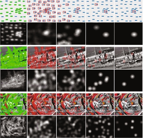
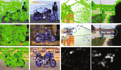
Figure 2.1 further shows the effect of tuning both contextual and mean shift scales (in each contextual scale, we settle the mean shift scale by adding 30 additional pixels) to achieve local-to-global context detections. Please note that tuning larger contextual and mean shift scales (e.g., to include all SIFT features into contextual representation) would result in focusing attention on viewing images. On the contrary, small contextual and mean shift scales degenerate CASL into a traditional local feature detector (e.g., SIFT [9]).
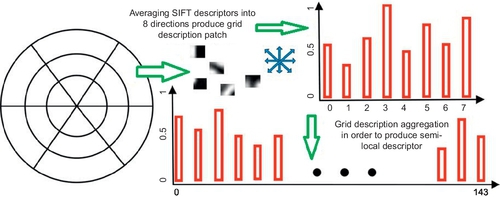
To further describe the detected feature, we follow the design of shape context: First, we provide a polar-grid division for context-aware description. A visualized example of our descriptor is shown in Figure 2.2. For each semi-local interest point, we include the local features in its δContext neighbor into its description. We subdivide these δContext neighbors into log-polar grids with 3 bins in radial directions (radius: 6, 11, and 15 pixels) and 6 in angular directions (angle: 0°, 60°, 120°, 180°, 240°, and 300°). It results in a 17-bin division. The central bin is not divided in angular directions to offer a certain robustness against feature locating precisions, which differs from GLOH [10]. In each grid, the gradient orientations of SIFT points are averaged and quantized in 8 bins. It produces a (3 × 6 × 8) 144-bin histogram for each CASE descriptor.
2.3.2 Comparison to Saliency
Different from the traditional local salient region detectors [8, 29, 80, 81], our semi-local detector can discover salient regions based on the DoCG field construction, which is a key advantage compared to the current works. Indeed, we have discovered that the high response locations for DoCG shares good similarity to visual saliency detection results. We explain this phenomenon from the construction process of the DoCG field: For a given location, our semi-local contextual measurement is derived by accumulating differences of co-occurrence strengths among K contextual scales. Similarly, the principle of a spatial saliency map [94] adopts a center-surround difference operation to discover highly contrasted points at different scales with Gaussian smoothing, which are then fused to evaluate point saliency. From another viewpoint, the DoCG field also shares certain similarity with the spectral saliency map [96] built by the Fourier transform, which retains the global spectrum phase to evaluate pixel saliency. In comparison, based on spatial convolution and difference accumulation, our DoCG field also preserves global character in general, for which the high-frequency fluctuations are discarded by spatial Gaussian convolutions over local feature densities, and the influences of frequency variances are further weakened by the different operations of contextual strengths. Notably, the “center-surround” operation is the basic and fundamental form of “context”, which is similar to many “center-surround” saliency detection operations [94].
2.4 Detector Learning
We further extend our detector design from the unsupervised case to the supervised case. In such a case, different from the traditional local feature detectors that perform in an unsupervised manner, our CASL detector also enables learning-based detection when there are multiple images available from an identical category.
In this setting, multiple images from the same category are available, which are treated as a whole in detection. For each image within this given category, we integrate semi-local statistics from other images to “teach” the CASL detector to locate category-aware semi-local peaks, which removes the features that are useless in discriminating this category from the others. This is achieved by refining the mean shift kernels and weights in the second phase of our CASL detector.
First, we adopt k-means clustering to group local features extracted from (1) the category images, or (2) the entire image dataset containing categories (if other images are also available). Subsequently, we build a bag-of-visual-words [16] model from the clustering results to produce a visual word signature for each local feature. For each visual word, its term frequency (TF) [28] weighting is calculated to describe its importance (within this category) in constructing SDoCG. This importance modifies the weight w(SDoCGi) and kernel GH(SDoCGi −SDoCG) in the mean shift search (Equation (2.1)). Figure 2.3 shows some detection examples.
To determine the mean shift search weight in Equation (2.1), the following modification is made:
in which the ith local feature belongs to the jth visual word; nj represents the number of local features that both belong to the jth visual word and are within the current image category; and NTotalC represents the total number of local features that are extracted from images of this category.
Given the labels of images belonging to the other categories, we further incorporate inter-category statistics, together with the former intra-category statistics, to build our learning-based CASL detector. This is achieved by introducing an inverted document weighting scheme [28] to improve the w(SDoCGi) in Equation (2.6):
in which NTotal represents the number of SIFT features extracted from the entire image database, which contains multiple image categories (the current category C is one of these categories).
The learning is achieved by refining the mean shift search kernel in Equation (2.6). The following modifications are made onto the positive definite bandwidth matrix H, which is simplified as a diagonal matrix ![]() (d is the dimension of the local feature descriptors, such as 128 for SIFT) into:
(d is the dimension of the local feature descriptors, such as 128 for SIFT) into:
The weight wF for each dimension hi is determined by Fisher discriminant analysis [98] as:
where wFi denotes the weight for the ith dimension di and DBetween and DWithin represent the between-category distance and within-category distance, respectively. We estimate the mean value of the ith dimension from both images within this category (mi) and images randomly sampled outside this category (m′i) with the same volume (denoted as Nc in Equation (2.4)). These values are then subdivided to obtain DBetween (calculated by (mi −m′i)(mi −m′i)). Similarly, the variance of this dimension is obtained as its averaged intra-category distance (![]() ).
).
We briefly review the connection between the proposed supervised CASL and other feature learning schemes as follows:
• Former works in learning-based local feature representation can be categorized into two groups. The first group aims to learn local feature descriptors [22, 23], which uses a ground truth set of matching correspondences (pairs of matched features) to learn descriptor parameters. Due to the requirement of “exact” matching correspondences, works in [22, 23] can be viewed as a strongly supervised learning scenario. On the contrary, our learning-based CASL only requires image category information rather than exact matching correspondences and hence can be viewed as a weakly supervised learning scenario.
• The second group derives from the frequent visual pattern mining [71, 72, 97], which adopts spatial association rules to mine frequent patterns (defined as certain spatial combinations of visual words in [71, 72, 97]). Our main advantages lie in the efficiency: Works in [71, 72, 97] all require the time-consuming frequent item set mining, such as the A-prior co-location pattern mining [99], to find meaningful patterns.
• Last and most important, our approach puts forward the learning mechanism into the feature detection step (mean shift over DoCG), which enables us to discover category-aware locations during feature detection. This differs from all related works in learning-based description [22, 23] or feature selection [71, 72, 97].
2.5 Experiments
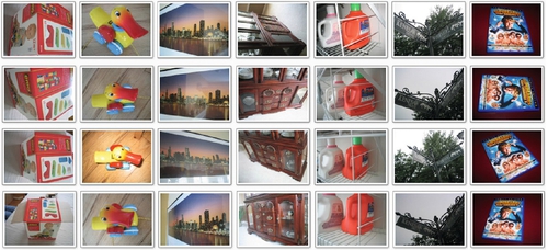
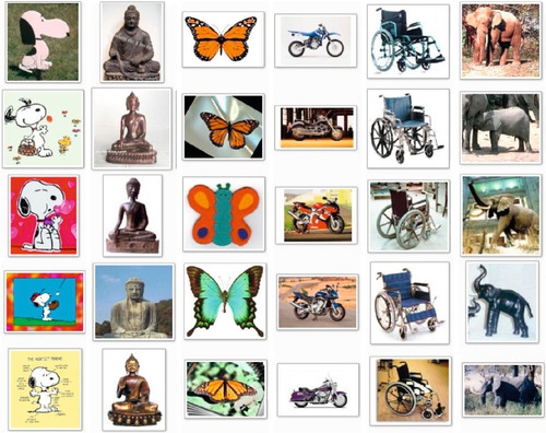
This section presents the quantitative experimental evaluations of our CASL detector with comparisons to current approaches. First, to prove that our CASL detector can still maintain good detection repeatability without regard to photometric variations, we give a series of standardized evaluations in the INRIA detector evaluation sequences [100]. Second, to demonstrate our effectiveness in discovering discriminative and meaningful interest points, we evaluate our CASL detector in two challenging computer vision tasks: (1) near-duplicated image retrieval in UKBench [16] as shown in Figure 2.4 and (2) object categorization in Caltech101, as shown in Figure 2.5.
2.5.1 Database and Evaluation Criteria
Despite detecting meaningful and discriminative salient regions, we should still ensure that our CASL detector can well retain the detector repeatability requirement [100], which is crucial for many computer vision applications, such as image matching and 3D scene modeling. We evaluated our detector repeatability in the INRIA detector evaluation sequences [100]. Using this database, we directly got the results reported in [100] as our baselines. In [100], the repeatability rate of detected regions among a test image t and the ith image in the test sequence are calculated as:
in which the |RI(![]() )| denotes the number of
)| denotes the number of ![]() repeatable [100] salient regions between t and i and the nt and ni represents the number of salient regions detected in the common part of images t and i, respectively. Refer to [100] for detailed experimental setups.
repeatable [100] salient regions between t and i and the nt and ni represents the number of salient regions detected in the common part of images t and i, respectively. Refer to [100] for detailed experimental setups.
We adopted the UKBench benchmark database [16] to evaluate the effectiveness of our CASL detector in the near-duplicated image retrieval task. The UKBench database contains 10,000 images with 2,500 objects. There are four images per object to offer sufficient variances in viewpoints, rotations, lighting conditions, scales, occlusions, and affine transforms.
We built our retrieval model over the entire UKBench database. Then we selected the first image per object to form a query set to test our performance. This experimental setup is identical to [16], which directly offers us the baseline performance of MSER + SIFT reported in [16]. Identical to [16], we ensured that the top returning photo would be the query itself, hence the performance depends on whether the system can return the remaining three photos of this object as early as possible. This criterion was measured as the “Correct Returning” in [16].
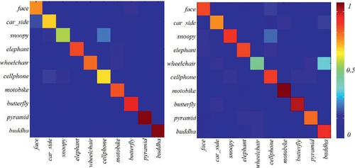
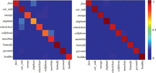
We selected a 10-category subset of Caltech101 database to evaluate our CASL detector in the object categorization task, including face, car side, snoopy, elephant, wheelchair, cellphone, motorbike, butterfly, pyramid, and buddha. Each image category contains approximately 60 to 90 images. We randomly selected 10 images from each category to form a test set, and used the rest of the images to train the classifiers.
We evaluated our categorization performance by measuring the percentage of corrected categorizations in each category (averaged hit/miss of its 10 test examples) to draw a categorization confused matrix.
There are five groups of baselines in our experimental comparisons.
1. Local Detectors: First, we offer four baselines of local detectors, including DoG [8], MSER [29], Harris-Affine [80], and Hessian-Affine [81].
2. Local Descriptors: Second, we offer two baselines of local descriptors, i.e., SIFT [9] and GLOH [10] (for comparison to the CASE descriptor).
3. Saliency Map Pre-Filtering: In both comparisons, we also compare with the saliency map pre-filtering [94] to select salient local features.
4. Integration of Category Learning: Third, we compare our learning-based CASL detector + SVM with two baselines of both CASL (without learning) + SVM and Bag-of-Visual-Words (SIFT) + SVM in the object categorization task.
5. Context-Aware Features: Finally, we compare our framework with two context-aware feature representations: (1) the “S1-C1-S2-C2” global contextual features [95] and (2) the Shape Context features [19] in both Caltech6 and Caltech101 recognition benchmark databases.
2.5.2 Detector Repeatability
Figure 2.6 shows the quantitative evaluations of the detector repeatability comparisons in the sequences of different scales, viewpoints, blurs, compressions, and illuminations. We can see that our CASL detector produces more repeatable detection results in the repeatability comparisons of compressions, illuminations, and blurs. And we obtain comparable performances in the repeatability comparisons of viewpoints and scales. Although our CASL detector produces generally fewer salient regions compared with the alterative approaches, we still achieve comparable performance by including semi-local spatial layouts in detection. Such spatial layout prevents unstable detections that are frequently found in traditional local feature detectors.
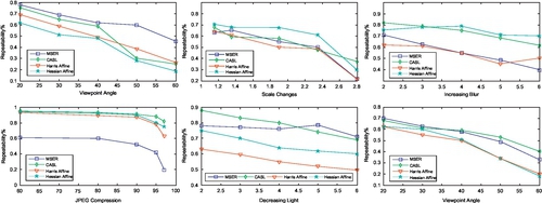
Figure 2.6 shows the quantitative evaluations of the detector repeatability comparisons in the sequences of different scales, viewpoints, blurs, compressions, and illuminations. We can see that, in many cases, our CASL detector produces more repeatable detection results in the repeatability comparisons of illuminations (fifth subfigure) and viewpoints (sixth subfigure); in all cases better in the repeatability comparisons of compressions (fourth subfigure); and in some cases better in the repeatability comparisons of blurs (third subfigure). However, we should note that we almost rank persistently worse than the Hessian-affine in viewpoints (first subfigure) and scales (second subfigure) (Hessian-affine is shown as one of the most effective detectors in the literature). One reason for this performance is that our CASL detector generally produces fewer salient regions, compared with the alternative approaches. In summary, our CASL detector achieves comparable performance to current detectors with generally fewer features per image. It could be due to including semi-local spatial layouts into detection. Such spatial layout prevents unstable detections that are frequently found in the traditional local features detectors. However, as shown in Figure 2.6, in some cases such as viewpoints or scales changes, Hessian-affine and MSER would be a better choice due to their simplicity.
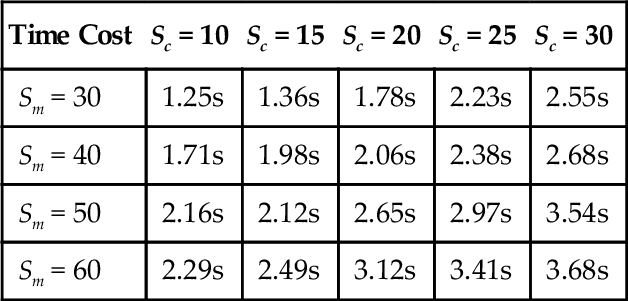
We further compare the computational time cost of our CASL detector with respect to different contextual scales and mean shift scales in Table 2.1. One interesting observation here is that by increasing both contextual and mean shift scale, the overall computational cost will subsequently increase.

2.5.3 CASL for Image Search and Classification
Note that in all methods, the “correct returning” is larger than 1, since the query would definitely find itself in the database. This experimental setup is identical to [16], which directly offers us the baseline performance of MSER + SIFT reported in [16]. We provide three implementation approaches: CASL (local detector part: DoG + SIFT) + SIFT, CASL (local detector part: MSER + SIFT) + SIFT, CASL (local detector part: DoG + SIFT) + CASE, CASL (local detector part: MSER + SIFT) + CASE; CASL (local detector part: DoG + MOP) + CASE, CASL (local detector part: MSER + MOP) + CASE. The experimental results show that in the local feature building block of CASL, the DoG + SIFT is a better choice for the task of near-duplicated image retrieval.
We built a 10-branch, 4-layer dictionary tree (VT) [16] for the UKbench database, which produced approximately 10,000 visual words. Nearly 450,000 CASL features and nearly 1,370,000 MSER + SIFT features were extracted from the entire database to build two vocabulary tree models [16], respectively (with inverted document indexing), each of which gave a bag-of-visual-words (BoW) vector [16] for each image. In the vocabulary tree model, if features within a node were less than a given threshold (100 for CASL features, 250 for SIFT features), we stopped the k-means division of this node, whether it had reached the deepest level or not. For a a-branch VT with m words, the search time for one feature point is aloga(m), which is proportional to the logarithm of branch number, and is independent of the database volume.
Figure 2.7 shows the performance of CASL + CASE in comparison with state-of-the-art local feature detectors (DoG, MSER), descriptors (SIFT), and the improvement based on saliency map pre-filtering:
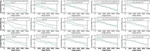
1. DoG [8] + SIFT [9], a widely adopted approach to building a bag-of-visual-words model.
2. MSER [29] + SIFT [9], which is the implementation of a vocabulary tree model [16] in near-duplicated search.
3. Saliency map [94] + MSER [29] + SIFT [9], in which we maintain only salient local features (measured by pixel-level saliency for a detected local feature location) to build the subsequent dictionary.
4. CASL + SIFT [9], which quantize the performance of our CASE descriptor.
5. DoG + MOP [21] as an alternative approach for our implemental baseline of DoG + SIFT [9]. However, as shown in Figure 2.7, this is a suboptimal choice for our subsequent CASL feature construction.
6. MSER [29] + MOP [21] as another alternative approach for our implemental baseline of DoG + SIFT [9]. Similarly, as shown in Figure 2.7, this is also a suboptimal choice for our subsequent CASL feature construction.
All these methods are based on the bag-of-visual-words quantization in which we adopt an inverted document search to find the near-duplicated images of the query example (in our query set) on the UKBench database.
From Figure 2.7, it is obvious that our CASL feature outperforms baseline methods that are based solely on local features with saliency map pre-filtering. Meanwhile, comparing with MSER [29], DoG [8] performs much better in building our local feature context.
Higher precisions also indicate two merits of our CASL detector: (1) More repeatability over rotation, scale, and affine transformations, which are common in the UKBench database; and (2) more discrimination within different object appearances. The photos in UKBench usually contain different objects such as CD covers with identical or near duplicated backgrounds. Hence, the capability to discriminate a foreground object from background clutter is essential for high performance.
For the task of object recognition, we built a 2-layer, 30-branch vocabulary tree [16] for image indexing, which contains approximately 900 visual words for this categorization task. For each category, the bag-of-visual-words vectors (approximately 900 dimensions for each image) are extracted for training. We offline built a SVM for every two categories. In the online recognition, we adopted a one-vs-one strategy to vote for the category membership for a test image: If one category won a SVM between this category and another category, we increased the voting score for the winning category by one. The category with the highest scores was assigned to the test image as its final label. Since we aimed to compare CASL with other detectors, we simply adopted a one-vs-one SVM in the classifier phase, which can be easily replaced by other sophisticated methods, e.g., SVM-KNN. We used the same parameter tuning approach described for near-duplicated image retrieval to tune the best contextual and mean shift scales.
Figures 2.8–2.9 present the confused matrix of different combination schemes, including (1) Saliency map + MSER + SIFT + SVM, (2) CASL (local features: MSER + SIFT) + CASE + SVM, (3) CASL (local features: DoG + SIFT) + CASE + SVM, and (4) learning-based CASL (local features: DoG + SIFT) + CASE + SVM. Generally speaking, CASL features perform much better than the approach that adopted saliency map pre-filtering to integrate semi-local cues. Meanwhile, the integration of learning part into CASL detector can largely boost the categorization performance in our current settlement.
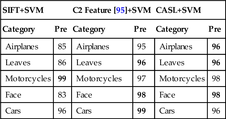
We give quantitative comparisons to the context-aware global features [95]. Identical to the settlement of [95], the Caltech5 is adopted in comparison. The performances of SIFT and C2 are directly from [95], the former of which adopted approximately 1,000-dimension features for categorization. To offer comparable evaluations, we built a CASL-based BoW vector containing about 900 visual words, and adopted linear SVM for classifier training. Note that we also used learning-based CASL in feature extraction.
Based on the comparison in the Caltech5 database (Table 2.2), our CASL detector achieved almost identical performance to the best performance reported in [95]. Since C2 +SVM already achieves very high (nearly 100 percent) performance, it is hard to obtain much better performance with a large margin. On the contrary, in addition to (slightly) better performance for C2 features, our CASL detector also shows much better results than SIFT + SVM with a large margin. Nevertheless, the C2 feature is better at higher computational cost. However, there are two major differences between our approach and the S1-C1-S2-C2 features [95]:
Table 2.2
Quantitative comparisons to contextual global features in Caltech5 subset
| SIFT+SVM | C2 Feature [95]+SVM | CASL+SVM | |||
| Category | Pre | Category | Pre | Category | Pre |
| Airplanes | 85 | Airplanes | 95 | Airplanes | 96 |
| Leaves | 86 | Leaves | 96 | Leaves | 96 |
| Motorcycles | 99 | Motorcycles | 97 | Motorcycles | 98 |
| Face | 83 | Face | 98 | Face | 98 |
| Cars | 96 | Cars | 99 | Cars | 96 |
First, the S1-C1-S2-C2-like feature extraction and classification framework [95] produces one feature vector per image with fixed feature dimension. This is different from our CASL detector that outputs patch-based features to produce bag-of-(semi-local)-word representations.
Second, the S2-C2 part in [95] needs training for prototype learning, which is indispensable in feature construction. In contrast, our CASL feature can also perform in an unsupervised manner (the learning is an optional choice), which can be easily reapplied into other unsupervised scenarios, and can be further combined with more complicated classifiers in the subsequent categorization step.
Regarding the polar-bin division strategy, there exists similarity between our CASE descriptor and the shape context feature [19]. Hence, it is a natural to replace our CASE descriptor with the shape context descriptor. Table 2.3 presents the experimental comparisons of our CASL + CASE feature with the CASL + shape context feature [19]. We should note that the shape context is a feature descriptor, which is not competitive but comprehensive to our CASL detector. However, we have found that the direct replacement of the shape context feature to our CASE descriptor cannot achieve satisfactory results for our CASL detections. Its similarity matching mechanisms are originally designed for shape primitives (Table 2.4).
Table 2.3
Quantitative comparisons to Shape Context in Caltech5 subset (classification phase: SVM)
| SIFT | CASL+Shape Context | CASL+CASE | |||
| Category | Pre | Category | Pre | Category | Pre |
| Airplanes | 85 | Airplanes | 92 | Airplanes | 96 |
| Leaves | 86 | Leaves | 86 | Leaves | 96 |
| Motorcycles | 99 | Motorcycles | 88 | Motorcycles | 98 |
| Face | 83 | Face | 84 | Face | 98 |
| Cars | 96 | Cars | 89 | Cars | 96 |
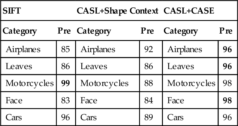
Table 2.4
Time cost comparisons of different contextual scales (Sc) and mean shift scales (Sm)
| Time Cost | Sc = 10 | Sc = 15 | Sc = 20 | Sc = 25 | Sc = 30 |
| Sm = 30 | 1.25s | 1.36s | 1.78s | 2.23s | 2.55s |
| Sm = 40 | 1.71s | 1.98s | 2.06s | 2.38s | 2.68s |
| Sm = 50 | 2.16s | 2.12s | 2.65s | 2.97s | 3.54s |
| Sm = 60 | 2.29s | 2.49s | 3.12s | 3.41s | 3.68s |
Based on the above three groups of experiments with comparisons to current technology, we have the following statements and guidelines about our application scenarios:
(1) What vision tasks are more suitable for CASL than traditional local feature detectors?
• The vision tasks emphasize discovering meaningful and discriminative features, rather than repeatable detection. For instance, generalized or specialized object recognition, image annotation, semantic understanding, and video concept detection.
• CASL is also suitable for the case where more attentional focus is needed, such as to describe images based solely on the most salient objects, or to discriminate foreground objects from backgrounds from a set of training images. In the latter case, we should also know their category labels beforehand to carry out our learning-based CASL.
(2) What scenarios are not as suitable for CASL instead of local feature detectors?
• When the vision tasks emphasize the repeatable detection more, rather than semantic or attentional discriminability, e.g., image matching and wide baseline matching.
• When the target image contains large amount of local features, and there are no demands to differentiate the foreground object from background clutter. For instance, scene matching and near-duplicated scene identification.
2.6 Summary
This chapter gave a systematic exploration of context information in designing interest point detector. Going beyond current approaches, we integrated contextual cues to enhance the interest point detector from a traditional local scale to a “semi-local” scale, which enabled us to discover more meaningful and discriminative salient regions without losing detector repeatability. Our other contribution here was to introduce a learning-based detector mechanism. It introduces the category learning (traditionally in subsequent classifier phases) into the feature detection phase, which locates category-aware interest points to improve performance of the subsequent recognition classifiers.
All of these contributions are integrated within a novel context-aware semi-local (CASL) feature detector framework, which is a two-step procedure: The first step builds the local feature context-based on a proposed difference of contextual Gaussians DoCG field, which offers the capability to highlight attentional salient regions, sharing good similarity with the saliency map detection results. The second step adopts a mean shift search to locate semi-local DoCG peaks as context-aware salient regions. This step naturally enables learning-based detection by integrating category learning into the mean shift weights and kernels. We conducted quantitative comparisons on image search, object categorization, and detector repeatability evaluations. We compared our performance with current approaches, based on which we further discussed the suitable and unsuitable scenarios for deploying our CASL detector.
Two interesting questions remain: First, we would further integrate category learning into the DoCG construction phase, in which we can adopt category-aware distributions to supervise the contextual representation of local features. Second, we are interested in extending our CASL feature to detect context-aware 3D salient regions within videos, in which we would investigate whether the sequential characteristics of successive frames can be used to construct the spatiotemporal contextual statistics in our first phase. The related work of this chapter is published in ACM Transactions on Intelligent Systems and Technology.