
Supervised Dictionary Learning via Semantic Embedding
Abstract
The visual dictionary and its indexing structure serves as the core of visual local representation systems. In Section 4.2, learning-based local interest-point detectors are investigated. Subsequently, Section 4.2.1 investigates the problem of unsupervised visual dictionary learning. However, as stated before, the building of a human visual system typically involves heavy learning procedures, either on the evolution of mankind or during growth of individual people. In other words, environmental supervision performs an important role in the visual representation system of a human being. In this chapter, similar ideas are discussed to investigate the possibility of learning-based visual representation.
4.1 Introduction
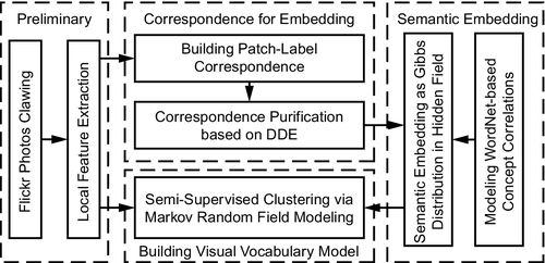
In this chapter, our overall target is to embed the semantic labels into the building procedure of the visual dictionary. To this end, there are two main issues that should be taken into consideration. First, how do we obtain a precise correspondence set between local image patches and semantic labels? This is hard to achieve via manual patch annotations in large-scale applications. We subsequently resort to collaborative image tagging on the Web. Second, how do we model correlative semantic labels to supervise the building of a visual dictionary? Given a set of local features with (partial) semantic labels, this chapter introduces a hidden Markov random field to model the supervision from correlative semantic labels to local image patches. Our model consists of two layers: The observed field layer contains local features extracted from the entire image database, where the visual metric takes effect to quantize the feature space into codeword subregions. The hidden field layer models (partial) semantic labels with WordNet-based correlation constraints. Semantics in the hidden field follow the Markov property to produce Gibbs distribution over local features in the observed field, which gives generative supervision to jointly optimize the local feature quantization procedure. For more detailed innovations and experimental validations, please refer to our previous publication in IEEE International Conference on Computer Vision and Pattern Recognition 2010. The overall framework is outlined in Figure 4.1.
4.2 Semantic Labeling Propagation
To feed into the proposed semantic embedding algorithms, we need a set of correspondences from local feature patches to semantic labels. Each correspondence offers a unique label and a set of local features extracted from photos with this label. In the traditional approaches, such patch-label correspondences are collected by either manual annotations or from the entire training image. For the latter case, labeling noises are an unaddressed problem in large-scale scenarios.
To handle this problem, we present a Density Diversity Estimation (DDE) approach to purify the patch-label correspondences collected from Flickr photos with collaborative labels. As a case study, we collected over 60,000 photos with labels from Flickr. For each photo, difference of Gaussians salient regions are detected and described by SIFT [9]. Each correspondence contains a label and a set of SIFT patches extracted from Flickr photos with this label. We discard infrequent labels in WordNet that contains less than 10 photos in LabelMe [103]. The remaining correspondences are further purified to obtain a ground truth correspondence set [104] for semantic embedding. This set includes over 18 million local features with over 450,000 semantic labels, containing over 3,600 unique words.
4.2.1 Density Diversity Estimation
Given a label si, Equation (4.1) denotes its initial correspondence set as < Di,si >, in which Di denotes the set of local features ![]() extracted from the Flickr photos with label si, and leji denotes a correspondence from label si to local patch dj:
extracted from the Flickr photos with label si, and leji denotes a correspondence from label si to local patch dj:
The first criterion of our filtering is based on evaluating the distribution density in local feature space. For a given dl, it reveals its representability for si. We apply nearest neighbor estimation in Di to approximate the density of dl in Equation (4.2):
where ![]() denotes the density for dl, which is estimated from its m nearest local patch neighbors in the local feature space of Di (for label si).
denotes the density for dl, which is estimated from its m nearest local patch neighbors in the local feature space of Di (for label si).
Another criterion of our filtering is based on evaluating the diversity of neighbors in dl. It removes the dense regions that are caused by noisy patches from only a few photos (such as meshed photos with repetitive textures). We adopt neighbor uncertainty estimation based on the following entropy measurement. For the same reason, we apply nearest neighbor estimation in Di to approximate the density of dl in Equation (4.2):
where ![]() represents the entropy at dl, nm is the number of photos that have patches within the m neighbors of dl, and ni is the total number of patches in photos with label si. Therefore, in local feature space, denser regions produced by a small fraction of the labeled photos will receive lower scores in our subsequent filtering in Equation (4.4).
represents the entropy at dl, nm is the number of photos that have patches within the m neighbors of dl, and ni is the total number of patches in photos with label si. Therefore, in local feature space, denser regions produced by a small fraction of the labeled photos will receive lower scores in our subsequent filtering in Equation (4.4).
Finally, we only retain the purified local image patches that satisfy the following DDE criterion:
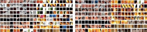
To interpret the above formulation, for a given label si, DDE selects the patches that frequently and uniformly appear within photos annotated by si. After DDE purification, we treat the purified correspondence set as a ground truth to build correspondence links leji from semantic label si to each of its local patches dj. Examples of the proposed DDE filtering is shown in Figure 4.2.
4.3 Supervised Dictionary Learning
4.3.1 Generative Modeling
We further present the proposed generative modeling for supervised dictionary learning. As shown in Figure 4.3, we introduce a hidden Markov random field (HMRF) model to integrate semantic supervision to quantize the local feature space. This model contains two layers:
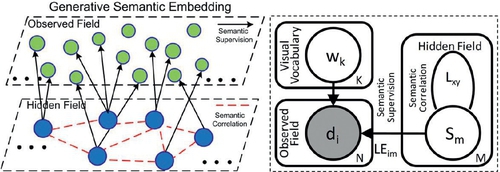
• As the first layer, a hidden field contains a graph of correlative nodes ![]() . Each si denotes a unique semantic label, which provides correspondence links (le) to a subset of local features in the observed field. Another type of link lij between two given nodes si and sj denotes their semantic correlation, which is measured by WordNet [105–107].
. Each si denotes a unique semantic label, which provides correspondence links (le) to a subset of local features in the observed field. Another type of link lij between two given nodes si and sj denotes their semantic correlation, which is measured by WordNet [105–107].
• As the second layer, an Observed Field contains local features ![]() extracted from the image database. Similarity between the two nodes follows a visual metric. Once there is a link leji from di to sj, we constrain di by sj from the hidden field with conditional probability P(di|sj).
extracted from the image database. Similarity between the two nodes follows a visual metric. Once there is a link leji from di to sj, we constrain di by sj from the hidden field with conditional probability P(di|sj).
Hence, feature set D is regarded as (partial) generative from the hidden field, and each di is conditionally independent given S:
Here, we set a hard quantization case, i.e., to assign a unique cluster label ci to each di. Therefore, D is quantized into a visual dictionary ![]() (corresponding feature vectors
(corresponding feature vectors ![]() ). The quantizer assignment for D is denoted as
). The quantizer assignment for D is denoted as ![]() . ci = cj = wk denotes di and dj belongs to an identical visual word wk. From Figure 4.3, the dictionary
. ci = cj = wk denotes di and dj belongs to an identical visual word wk. From Figure 4.3, the dictionary ![]() and the semantics S are conditionally dependent given the observed field, which thereby incorporates S to optimize the building of
and the semantics S are conditionally dependent given the observed field, which thereby incorporates S to optimize the building of ![]() .
.
In this chapter, we define a Markov random field on the hidden field, which imposes Markov probability distribution to supervise the quantizer assignments C of D in the observed field:
Here, x and y are nodes in the hidden field that link to points i and j in the observed field, respectively (lejx and leiy≠0). ![]() ′y is the hidden field neighborhood of y. The cluster label ci depends on its neighborhood cluster labels ({cj}). This “neighborhood” definition is within the hidden field (i.e., each cj is the cluster assignment of dj that has neighborhood labels (sx) within
′y is the hidden field neighborhood of y. The cluster label ci depends on its neighborhood cluster labels ({cj}). This “neighborhood” definition is within the hidden field (i.e., each cj is the cluster assignment of dj that has neighborhood labels (sx) within ![]() for sy of di).
for sy of di).
Considering a particular configuration of quantizer assignments ![]() (which gives a “visual dictionary” representation), its probability can be expressed as a Gibbs distribution [108] generated from the hidden field, depending on the following Hammersley-Clifford theorem [109]:
(which gives a “visual dictionary” representation), its probability can be expressed as a Gibbs distribution [108] generated from the hidden field, depending on the following Hammersley-Clifford theorem [109]:
where ![]() is a normalization constraint and
is a normalization constraint and ![]() is the overall potential function for the current quantizer assignment C, which can be decomposed into the sum of potential functions
is the overall potential function for the current quantizer assignment C, which can be decomposed into the sum of potential functions ![]() for each visual word wk, which only considers influences from points in wk (volume
for each visual word wk, which only considers influences from points in wk (volume ![]() ).
).
To interpret the above calculation and formulation, let say two data points di and dj in wk contribute to ![]() if and only if: (1) correspondence links lexi and leyj exist from di and dj to semantic nodes sx and sy, respectively; and (2) semantic correlation lxy exists between sx and sy in the Hidden Field.
if and only if: (1) correspondence links lexi and leyj exist from di and dj to semantic nodes sx and sy, respectively; and (2) semantic correlation lxy exists between sx and sy in the Hidden Field.
To solve it, we adopt the WordNet:Similarity [106] to measure lxy, which is constrained to [0,1] with lxx = 1. A large lxy means a close semantic correlation (usually from correlative nouns, e.g., “rose” and “flower”). In Equation (4.4), we subtract the sum of lxy to fit the potential function ![]() . Intuitively, P(C) gives higher probabilities to the quantizer that follows semantic constraints better. We calculate P(C) by:
. Intuitively, P(C) gives higher probabilities to the quantizer that follows semantic constraints better. We calculate P(C) by:
4.3.2 Supervised Quantization
Overall, to achieve semantic embedding, we have ![]() in the observed field as generative from a particular quantizer configuration
in the observed field as generative from a particular quantizer configuration ![]() through its conditional probability distribution P(D|C):
through its conditional probability distribution P(D|C):
Therefore, given ci, the probability density P(di,vk) is measured by the visual similarity between feature point di and its visual word feature vk. To obtain the best C, we investigate the overall posterior probability of a given C as P(C|D) = P(D|C)P(C), in which we consider the probability of P(D) as a constraint. Finding maximum-a-posterior of P(C|D) can be converted to maximizing:
Subsequently, two criteria are there to optimize the quantization configuration C (and hence the dictionary configuration ![]() ): (1) The visual constraint P(D|C) imposed by each point di to its corresponding word feature vk, which is regarded as the quantization distortions of all visual words:
): (1) The visual constraint P(D|C) imposed by each point di to its corresponding word feature vk, which is regarded as the quantization distortions of all visual words:
and (2) The semantic constraints P(C) imposed from the hidden field, which are measured as:
It is worth noting that, due to the constraints in P(C), MAP cannot be solved as a maximum likelihood. Furthermore, since the quantizer assignment C and the centroid feature vectors ![]() could not be obtained simultaneously, we cannot directly optimize the quantization in Equation (4.6). We address this by a k-means clustering, which works in an estimation maximization manner to estimate the probability cluster membership. The E step updates the quantizer assignment C using the MAP estimation at the current iteration. Different from traditional k-means clustering, we integrate the correlations between data points by imposing
could not be obtained simultaneously, we cannot directly optimize the quantization in Equation (4.6). We address this by a k-means clustering, which works in an estimation maximization manner to estimate the probability cluster membership. The E step updates the quantizer assignment C using the MAP estimation at the current iteration. Different from traditional k-means clustering, we integrate the correlations between data points by imposing ![]() to select configuration C. The quantizer assignment for each di is performed in a random order, which assigns wk to di and minimizes the contribution of di to the objective function. Therefore,
to select configuration C. The quantizer assignment for each di is performed in a random order, which assigns wk to di and minimizes the contribution of di to the objective function. Therefore, ![]() . Without losing generality, we give a log estimation from Equation (4.6) to define the Obj(ci|di) for each di as follows:
. Without losing generality, we give a log estimation from Equation (4.6) to define the Obj(ci|di) for each di as follows:
The M step re-estimates the K cluster centroid vectors ![]() from the visual data assigned to them in the current E Step, which minimizes Obj(ci|di) in Equation (4.9) (equivalent to maximizing the expects of “visual words”). We update the kth centroid vector vk based on the visual data within wk:
from the visual data assigned to them in the current E Step, which minimizes Obj(ci|di) in Equation (4.9) (equivalent to maximizing the expects of “visual words”). We update the kth centroid vector vk based on the visual data within wk:
Single-Level Dictionary: Algorithm 4.1 presents the building flow of a single-level dictionary. Our time cost is almost identical to the traditional k-means clustering. The only additional cost is the nearest neighbor calculation in the hidden field for P(C), which can be performed using an o(m2) sequential scanning for m semantic labels (each with a heap ranking) and stored beforehand.
Algorithm 4.1
Building a Supervised Visual Dictionary
Hierarchical Dictionary: Many large-scale retrieval applications usually involve tens of thousands of images. To ensure online search efficiency, hierarchical quantization is usually adopted, e.g., vocabulary tree (VT) [16], approximate k-means (AKM) [24], and their variations. We also deploy our semantic embedding to a hierarchical version, in which the vocabulary tree model [16] is adopted to build a visual dictionary based on hierarchical k-means clustering. Compared to single-level quantization, the vocabulary tree model pays extreme attention on the search efficiency: To produce a bag-of-words vector for an image using a w-branch m-word VT model, the time cost is ![]() , whereas using a single-level word division, the time cost is O(m). During hierarchical clustering, our semantic embedding is identical within each subcluster.
, whereas using a single-level word division, the time cost is O(m). During hierarchical clustering, our semantic embedding is identical within each subcluster.
4.4 Experiments
We give two groups of quantitative comparisons in our experiments. The first group shows the advantages of our generative semantic embedding (GSE) to the unsupervised dictionary construction schemes, including comparisons to (1) the traditional VT [16] and GNP, and (2) the GSE without semantic correlations (ignoring semantic links in the hidden field graph to infer P(C)). The second group compares our GSE model with two related works in building a supervised dictionary for object recognition tasks: (1) Class-specific adaptive dictionary [42], and (2) learning-based visual word merging [110]. During comparison, we also investigate how the dictionary sparsity, embedding strength, and label noise (these concepts will be explained later) affect our performance.
4.4.1 Database and Evaluations
In this chapter, two databases are adopted in evaluation: (1) The Flickr database contains over 60,000 collaboratively labeled photos, which gives a real-world evaluation for our first group of experiments. It includes over 18 million local features with over 450,000 user labels (over 3,600 unique keywords). For Flickr, we randomly select 2,000 photos to form a query set, and use the remaining 58,000 to build our search model. (2) The PASCAL VOC 05 database [111] evaluates our second group of experiments. We adopt VOC 05 instead of 08 since the former directly gives quantitative comparisons to [110], which is most related to our work. We split PASCAL into two equal-sized sets for training and testing, which is identical to the settlement in [110]. The PASCAL training set provides bounding boxes for image regions with annotations, which naturally gives us the purified patch-label correspondences.
4.4.2 Quantitative Results
In the Flickr database, we build a 10-branch, 4-level vocabulary tree for semantic embedding, based on the SIFT features extracted from the entire database. If a node has fewer than 2,000 features, we stop its k-means division, whether it has achieved the deepest level or not. A document list (approximately 10,000 words) is built for each word to record which photo contains this word, thus forming an inverted index file. In the online processing, each SIFT feature extracted from the query image is sent to its nearest visual word, in which the indexed images are picked out to rank the similarity scores to the query. As a baseline approach, we build a 10-branch, 4-level unsupervised vocabulary tree for the Flickr database. The same implementations are carried out for the PASCAL database, in which we reduce the number of hierarchical layers to 3 to produce a visual dictionary with visual word volume ≈ 1,000.
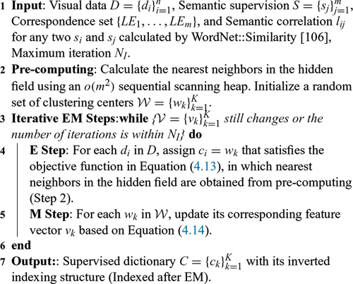
Similar to [42], it is informative to look at how our semantic embedding affects the averaged ratios between inter-class and intra-class distances. The inter-class distance is the distance between two averaged BoW vectors: one from photos with the measured semantic label, and one from random-select photos without this label; the intra-class distance is the distance between two BoW vectors from photos with an identical label. Our embedding ensures that nearby patches with identical or correlative labels would be more likely to quantize into an identical visual word. In Figure 4.4, this distance ratio would significantly increase after semantic embedding.
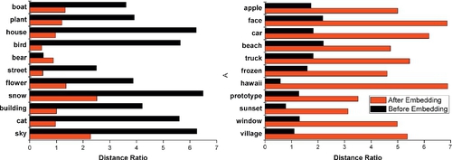
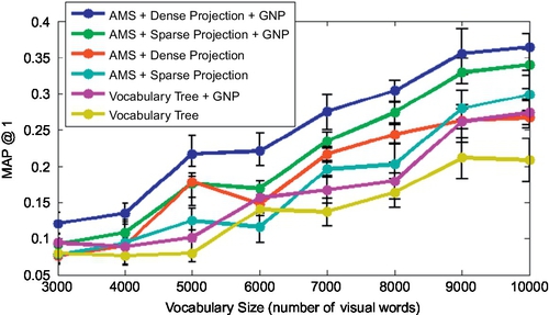
Figure 4.5 shows our semantic embedding performances in the Flickr database, with comparisons to both VT [16] and GNP [27]. With identical dictionary volumes, our GSE model produces a more effective dictionary than VT. Our search efficiency is identical to VT and much faster than GNP. In the dictionary building phase, the only additional cost comes from calculating P(C). Furthermore, we also observe that a sparse dictionary (with fewer features per visual word on average) gives generally better performance by embedding an identical amount of patch-label correspondences.
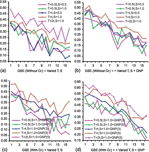
We explore semantic embedding with different correspondence sets constructed by (1) different label noise T (DDE purification strength) (original strength t is obtained by cross-validation) and (2) different embedding strength S (S = 1.0 means we embed the entire purified correspondence set to supervise the codebook, 0.5 means we embed half). There are four groups of experiments in Figure 4.6 used to validate our embedding effectiveness: (a) GSE (without hidden field correlations Cr.) + Varied T, S: It shows that uncorrelative semantic embedding does not significantly enhance MAP by increasing S (embedding strength), and degenerates dramatically with large T (label noise), mainly because the semantic embedding improvement is counteracted by miscellaneous semantic correlations. (b) GSE (without hidden field correlations Cr.) + Varied T, S + GNP: Employing GNP could improve MAP performance to a certain degree. However, the computational cost would be increased. (c) GSE (with Cr.) + Varied T, S: Embedding with correlation modeling is a much better choice. Furthermore, the MAP degeneration caused by large T could be refined by increasing S in large-scale scenarios. (d) GSE (With Cr.) + Varied T, S + GNP: We integrate the GNP in addition to GSE to achieve the best MAP performance among methods (a)–(d). However, its online search is time-consuming due to GNP (Figure 4.7).
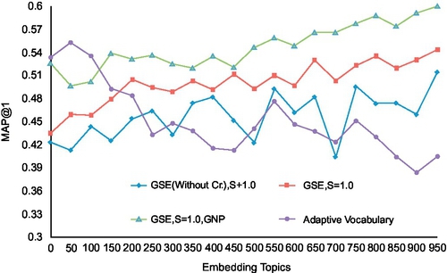
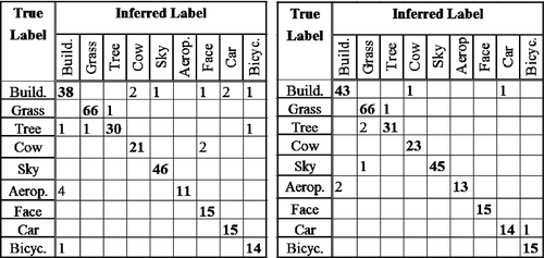
We compare our supervised dictionary with two learning-based vocabularies in [42, 110]. First, we show comparisons between our GSE model and the adaptive dictionary [42] in the Flickr database. We employed the nearest neighbor classifier in [110] for both approaches, which reported the best performance among alternative approaches in [110]. For [42], the nearest neighbor classification is adopted to each class-specific dictionary. It votes for the nearest BoW vector, assigning its label as a classification result. Not surprisingly, within limited (tens of) classes, the adaptive dictionary [42] outperforms our approach. However, putting more labels into dictionary construction will increase our search MAP. Our method can finally outperform the adaptive dictionary [42] when the number of embedding labels is larger than 171. In addition, adding new classes into the retrieval task would linearly increase the time complexity of [42]. In contrast, our search time is constant without regard to embedding labels. Second, we also compare our approach to [110] within the PASCAL VOC. We built the correspondence set based on the SIFT features extracted from the bounding boxes with annotation labels [111], from which we conducted the semantic embedding with S = 1.0. In classifier learning, each annotation is viewed as a class with a set of BoW vectors extracted from the bounding box with this annotation. Identical to [110], the classification of the test bounding box (we know its label beforehand as ground truth) is a nearest neighbor search process. Figure 4.8 shows that, in almost all categories, our method gives better precision than [110] within ten identical PASCAL categories.
4.5 Summary
This chapter presented a semantic embedding framework, which aims for supervised, patch-based visual representation from collaborative Flickr photos and labels. Our framework introduced a hidden Markov random field to generatively model the relationships between correlative Flickr labels and local image patches to build supervised dictionary. By simplifying the Markov properties in the hidden field, we showed that both unsupervised and supervised quantizations (without considering semantic correlations) can be derived from our model. In addition, we have published a patch-label correspondence set [104] (containing over 3,600 unique labels with over 18 million patches) to facilitate subsequent research of this topic.
One interesting issue remains open: For large-scale applications, the generality of the supervised dictionary needs further exploration. Transfer learning is a feasible solution to adapt a supervised dictionary among different scenarios, e.g., from scene recognition to object detection, which will be further considered in our future work. The related works based on this chapter were accepted as oral presentations in IEEE CVPR 2010, as well as in IEEE Transactions on Image Processing.