Investigation and Selection Procedure
Abstract
This chapter discusses the effects of mobile ad hoc black hole attacks in the networks. To achieve this, it simulated the mobile ad hoc network scenarios which include black hole node using NS Network Simulator program. To simulate the black hole node in a mobile ad-hoc network, this project implemented a new protocol that drops data packets after receiving them. In this section, having shown how it has tested the black hole implementation, it will present the simulations of black hole attack to demonstrate its effects. Then, it will evaluate the effects of black hole attacks on a mobile ad hoc network.
Keywords
Mobile ad hoc black hole attacks; NS Network Simulator program
4.1 Introduction
This chapter discusses the effects of mobile ad hoc black hole attacks in the networks. To achieve this, it simulated the mobile ad hoc network scenarios which include black hole node using NS Network Simulator program (Issariyakul & Hossain, 2012). To simulate the black hole node in a mobile ad hoc network, this project implemented a new protocol that drops data packets after receiving them. In this section, having shown how it’s tested with the black hole implementation, it will present the simulations of black hole attack to demonstrate its effects. Then, it will evaluate the effects of black hole attacks on a mobile ad hoc network.
4.2 Executing a New Routing Protocol in NS to Simulate Black Hole Behavior
Ros and Ruiz (2004) described the implementation of a new MANET unicast routing protocol in NS-2. The initial implementation of this project is based on the work of Ros and Ruiz (2004). In this research, nodes that exhibit black hole behavior in mobile ad hoc network using AODV routing protocol is used. Since the nodes behave as a black hole, they have to use a new routing protocol that can participate in the AODV messaging. Implementation of this new routing protocol is explained below in detail:
All routing protocols in NS are installed in the directory of “ns-2.35.” First and foremost, the AODV protocol found in this directory is being duplicated after which the directory is renamed as “blackholeaodv”. Names of all associated aodv files labeled as “aodv” in the directory are changed to “blackholeaodv,” that is, blackholeaodv.cc, blackholeaodv.h, blackholeaodv.tcl, blackholeaodv_rqueue.cc, blackholeaodv_rqueue.h, etc. in this new directory excluding “aodv_packet.h.” The main concept is such that AODV and black hole AODV protocols send the same AODV packets. Hence, we do not copy “aodv_packet.h” file into the blackholeaodv directory.
Changes have been made to all classes, functions, structs (except struct names that belong to AODV packet.h code), variables, and constants names in all the files in the directory. Also, the aodv and blackholeaodv protocols have been designed to send each other aodv packets. These two protocols are actually the same.
Following the above changes, two common files that are used in NS-2 globally to integrate new blackholeaodv protocol to the simulator have also been changed. In the work of Ros and Ruiz (2004), more files are changed to add new routing protocol and this new protocol uses its own packets. But in this research work, we do not need to add a new packet. Therefore, only two files were changed. The changes are explained below.
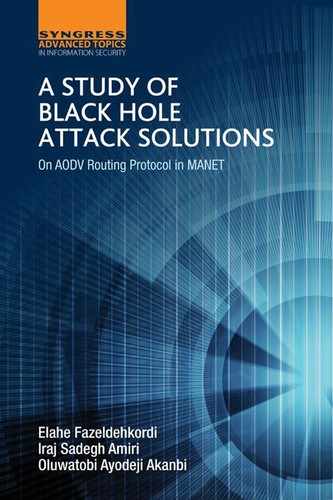
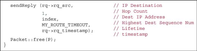
The First file modified is “ cllib s-lib.tcl” such that protocol agents are implemented as a procedure. In the case of the nodes using blackholeaodv protocol, this agent is scheduled at the beginning of the simulation and it is designated to the nodes that will use blackholeaodv protocol. The agent procedure for blackholeaodv is shown in Fig. 4.1:
Second file which modified is “makefile” in the root directory of the “ns-2.35.” After all implementations are ready, we have to compile NS-2 again to create object files. We have added the below lines in Fig. 4.2 to the “makefile.”

To this extent, implementation of a new routing protocol labelled as blackholeaodv have been done. But black hole behaviors have not yet been implemented in this new routing protocol. To include black hole behavior into the new AODV protocol, same changes were made in blackholeaodv/blackholeaodv.cc C++ file. Description of these changes made in blackholeaodv/blackholeaodv.cc file explaining working mechanism of the AODV and black hole AODV protocols are as below.
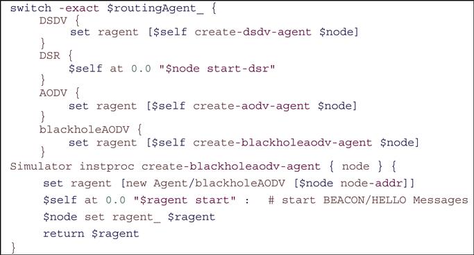
In a scenario where a packet is received by the “recv” function of the “aodv/aodv.cc,” the packets are being processed based on its type. In case the type of packet is associated with any of AODV route management packets, it sends the packet to the “recvAODV” function that will be explained below. If the received packet is a data packet, typically AODV protocol sends it to the destination address; on the other hand, behaving as a black hole, it drops all data packets as long as the packet does not come to itself. In the code below, the first “if” condition provides the node to receive data packets if it is the destination. The “else” condition drops all remaining packets. The “if” statement is shown in Fig. 4.3:
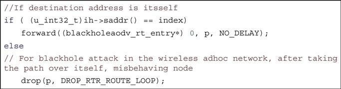
If the packet is associated AODV management packet, “recv” function sends it to “recvblackholeAODV” function. The “recvblackholeAODV” function checks the type of the AODV management packet and based on the packet type it sends them to appropriate function with a “case” statement. For instance, RREQ packets are sent to the “recvRequest” function, RREP packets to “recvReply” function, etc., and case statements of “recvblackholeAODV” function are shown in Fig. 4.4:
In our case, we will consider the RREQ function because black hole behavior is carried out as the malicious node receives an RREQ packet. When the malicious node receives an RREQ packet, it immediately sends RREP packet as if it has fresh enough path to the destination. Malicious node tries to deceive nodes sending such an RREP packet. Highest sequence number of AODV protocol is 4294967295, 32-bit unsigned integer value. Values of RREP packet that malicious node will send are described below. The sequence number is set to 4294967295 and hop count is set to the false RREP message of the black hole attack is shown in Fig. 4.5:
After all changes are finished, we have to recompile all NS-2 files to create object files. For recompiling, we should run make clean, then make depend, and finally make command in ns2.35 directory. Now, we have a new test bed to simulate black hole attack in AODV protocol. The next section will explain the simulations and simulation results.
4.3 Examining the Black Hole AODV
The implementation of the black hole is tested to see whether it is correctly working or not. To be sure the implementation is correctly working, we used the NAM (network animator) application of NS. To test the implementation, we used two simulations. In the first scenario, we did not use any black hole AODV node (the malicious node that exhibits the black hole attack will be called “black hole node”). In the second scenario, we added a black hole AODV node to the simulation. Then, we compared the results of the simulations using NAM.
4.3.1 Simulation Parameters and Measured Metrics
To take accurate results from the simulations, we used UDP protocol. The source node keeps on sending out UDP packets, even if the malicious node drops them, while the node finishes the connection if it uses TCP protocol. Therefore, we could observe the connection flow between sending node and receiving node during the simulation. Furthermore, we were able to count separately the sent and received packets since the UDP connection is not lost during the simulation. If we had used TCP protocol in our scenarios, we could not count the sent or received packets since the node that starts the TCP connection will finish the connection after a while if it has not received the TCP ACK packet.
It has generated 10 networks: 6, 20, 30, 40, 50, 60, 70, 80, 90, and 100 nodes, and then creates a UDP connection between node 0 and node 4 in all of scenarios and attach CBR (constant bit rate) application that generates constant packets through the UDP connection. CBR packet size is 512 bytes; data rate is set to 10 Kbyte/sec. Duration of the scenarios is 500 s and the CBR connections started at time 2.0 s and continue until the end of the simulation, in a 670×670-m flat space. The appropriate positions of the nodes are manually designed to show the data flow and also introduce movement for nodes 0–5 in network with 6 nodes and for nodes 0–9 for networks with 20 and for nodes 0–29 with 30 nodes that can observe the changes of the data flow in networks with different number of nodes. The Tcl script contains a black hole AODV for the first simulation is shown in Appendix A.
4.3.2 Appraisal of the Simulation
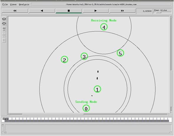
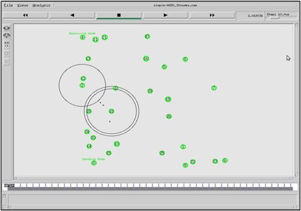
In the first scenario where there is not a black hole AODV node, connection between node 0 and node 4 is correctly flowed when look at the animation of the simulation, using nam.file. Figs. 4.6–4.11 show the data flow from node 0 to node 4 in three different networks with 6, 20, and 30 mobile nodes. Fig. 4.6 shows data flow for network with six nodes, the connection between node 0 and node 4 established via node 1.
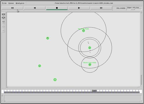
In the first network when node 1 leaves the propagation range of the node 0 while moving, the new connection is established via node 3. The new connection path is shown in Fig. 4.7:
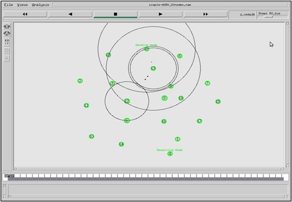
Fig. 4.8 shows data flow for network with 20 nodes, the connection between node 0 and node 4 established via nodes 13, 12, and 6:
In the second network when node 13 leaves the propagation range of the node after moving, the new connection is established via nodes 8, 17, 11, and 2. The new connection path is shown in Fig. 4.9:
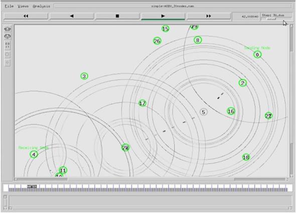
Fig. 4.10 shows data flow for network with 30 nodes, that connection between node 0 and node 4 established via nodes 18, 2, and 12:
In the third network when node 18 leaves the propagation range of the node after moving, the new connection is established via nodes 5, 28, and 10. The new connection path is shown in Fig. 4.11.
4.4 Simulation of Black Hole Attack
4.4.1 Simulation Parameters and Measured Metrics
Different scenarios are used in our work: 6, 20, 30, 40, 50, 60, 70, 80, 90, and 100 AODV nodes without black hole attack; 6, 20, 30, 40, 50, 60, 70, 80, 90, and 100 AODV nodes with one black hole node; and 6, 20, 30, 40, 50, 60, 70, 80, 90, and 100 AODV nodes with two black hole nodes. UDP connections are established between nodes. In all of the scenarios, the sending node is node 0 and the receiving node is node 4 and packets send from sending node to receiving node.
Node positions and movements are generated manually, during 500 s, in a 670×670-m space. The CBR application is attached that generates constant packets through the UDP connection. Duration of the scenarios is 500 s and the CBR connections started at time 2.0 s until end of scenario. In our scenarios, CBR parameters are as follows:
And it did not use random packets in the simulation. Nodes in the simulation are generated by the statements that are shown in Fig. 4.12. The first statement: “$ns_ node-config -adhocRouting blackholeAODV” changes AODV routing protocol to “blackholeAODV” that is implemented in NS, so we can easily add the black hole AODV behavior with writing the number of node we wish to be black hole. And second statement: “$ns_ node-config -adhocRouting AODV” creates AODV nodes (Fig. 4.13).
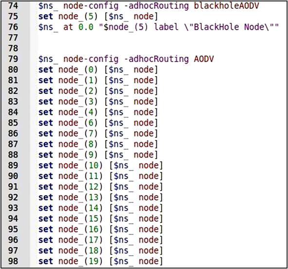
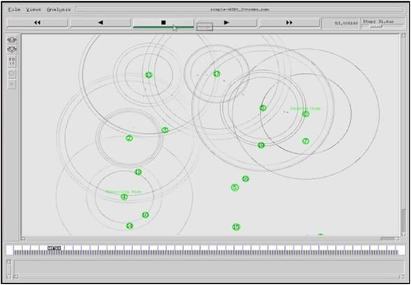
Our simulation files are named with their simulation number and “BlackHole” number, for example, “sim1for1BlackHole6Mobility.tcl,” “sim1for2BlackHole6Mobility.tcl”. To run the AODV simulation without black hole attack, we changed the “$val(nnaodv)” variable to 6, 20, 30, 40, 50, 60, 70, 80, 90, and 100 nodes in different scenarios and then put the comment “#” in front of the “$ns_ node-config -adhocRouting blackholeAODV” statement and then we copied the Tcl script in same directory changing “BlackHole” definition of the file name with “simple-AODV,” for example, “simple-AODV_6nodees.tcl” is used for AODV without black hole attack including six nodes. The content of the first simulation file of the black hole AODV is shown in Appendix A. Node 5 being a black hole AODV node absorbs the packets in the connection from node 0 to node 4. Figs. 4.14–4.16 show how the black hole AODV node attracts the traffic. In Fig. 4.14, node 5 is black hole node, node 0 is sending node, and node 3 is destination node. Node 5 sends RREP to sending node’s RREQ and after receiving data packets drop them:
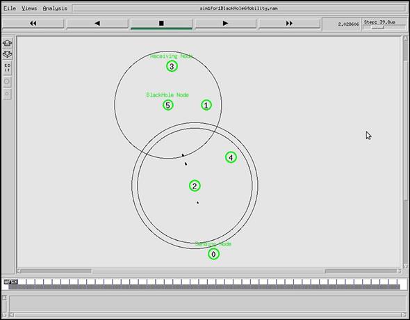
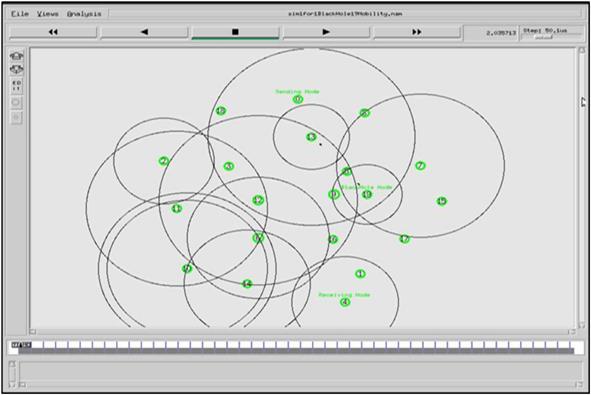
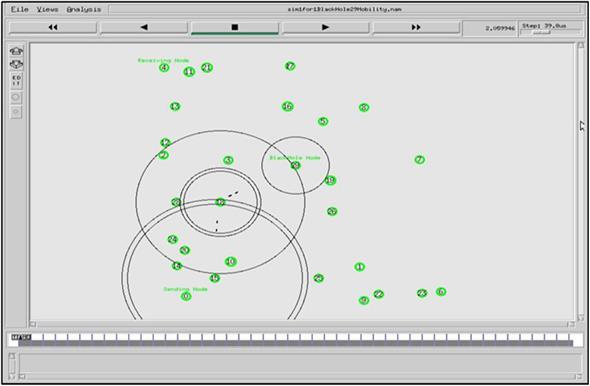
Fig. 4.15 shows same simulation with 20 nodes; in this examination, it’s supposed that node 19 is black hole node, node 0 is sending node, and node 4 is receiving node. As you can see, node 19 as a black hole node drops packets after receiving them:
Fig. 4.16 shows simulation with 30 nodes; in this examination as you can see node 29 as a black hole node drops packets after receiving them:
4.4.2 Testing the Trace File and Obtaining the Results
It has gotten the simulation result from output and finds documents of the Tcl scripts, which has “.tr” elongation. Then, it finds documents that include all events in the simulation such as “when the packets are dispatched?,” “which node generated them?,” “which node has received?,” “which type of package is dispatched?,” “if it is dropped why it is dropped?,” etc. In our simulations, we use “new-trace” document format that is particularly utilized in wireless networks and encompasses comprehensive happening information. The new-trace file experiment is shown in Appendix B. Its areas are explained in Appendix C.
To get the outcomes from the find files, we wanted only the event kind in area 0; node id (-Ni) and find the grade (-Nl) in area 4; and main address, destination address, and package sort in the area 5. To spot the on peak of facts and figures from the find document, we tend to use “cat” order of UNIX scheme and composed its outputs to a file for all find documents of the simulations. Of all the yields, we solely need “s” value of the happening facts and figures inside the area none, to count what number “cbr” packets “ar” dispatched by the causation node “r” worth of the happening data within the area 0, to enumerate how numerous CBR packets are obtained by the obtaining node “node id” worth of the node id information within the area 4, for the causation nodes or receiving nodes “MAC” worth of the find level information inside the area 4, to filter “MAC” level.
“Source Address” is values of the source and “Destination Address” is place visited by the address data in field 5, to count the packets that go from the dispatching node to the getting node. “cbr” value of the packet kind information within the field 5 to filter “cbr” packets.
To filter this information, we have a tendency to use “grep” command of the UNIX operating system reading the file developed by “cat” order and provided its output to word count (WC) order of the UNIX operating system as an input to count what quantity data have filtered and composed the end result to a new file. For demonstration; to count cbr packets the outcome by node 0 (sending node) the order “grep “s zero 0 --- 0.0 1.0 cbr” sim1forBlackHole.txt | wc -l >> result.txt” is utilized.
On other hand, to calculate “cbr” packets obtained by node 1 (receiving node), “grep ‘s 0 MAC --- 0.0 1.0 cbr’ sim1forBlackHole.txt | wc -l >> result.txt” is used. These commands are directed for all nodes within the all replication and are in writing as a batch file. Content of this file is shown in Appendix C.
4.4.3 Appraisal of Results
Three different simulations have examined. In the first one, every node is working in cooperation with each other to keep the network in communication. The second one has one malicious node and third one has two malicious nodes that carry out by black hole attack. In this study, the results of these three simulations are compared to understand the network and node behaviors.
First it evaluated the packet loss. We counted how many packets are sent by the sending nodes and how many of them reached the receiving nodes. Tables 4.1–4.4 compare the normal and black hole network for total drop packets, end-to-end delay, routing overhead, and packet delivery ratio.
Table 4.1
| Number of nodes | 6 | 20 | 30 | 40 | 50 | 60 | 70 | 80 | 90 | 100 |
| Before black hole attack | 0 | 0 | 0 | 0 | 0 | 0 | 0 | 0 | 0 | 0 |
| After one black hole attack | 498 | 498 | 498 | 498 | 498 | 498 | 498 | 498 | 498 | 498 |
| After two black hole attacks | 498 | 498 | 498 | 498 | 498 | 498 | 498 | 498 | 497 | 498 |
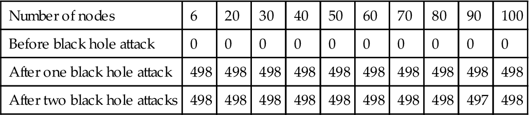
Table 4.2
| Number of nodes | 6 | 20 | 30 | 40 | 50 | 60 | 70 | 80 | 90 | 100 |
| Before black hole attack | 0.116364 | 0.116387 | 0.1059 | 0.101903 | 0.100342 | 0.100103 | 0.078637 | 0.078323 | 0.065856 | 0.0551 |
| After one black hole attack | 0 | 0.061414 | 0.0596 | 0 | 0 | 0 | 0.024322 | 0.0177599 | 0.017762 | 0 |
| After two black hole attacks | 0 | 0.023582 | 0.023923 | 0 | 0 | 0 | 0 | 0.017523 | 0.017482 | 0.017122 |
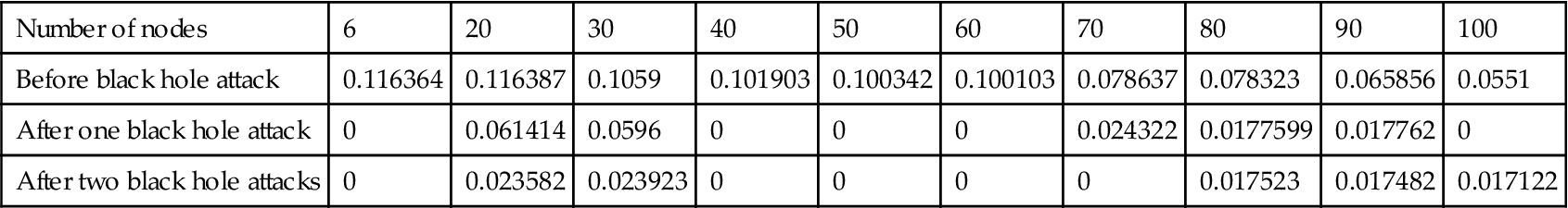
Table 4.3
| Number of nodes | 6 | 20 | 30 | 40 | 50 | 60 | 70 | 80 | 90 | 100 |
| Before black hole attack | 0.002 | 0.005 | 0.0089 | 0.01 | 0.015 | 0.014 | 0.016 | 0.024 | 0.026 | 0.029 |
| After one black hole attack | 0.001 | 0.01 | 0.009 | 0.016 | 0.017 | 0.018 | 0.02 | 0.024 | 0.026 | 0.03 |
| After two black hole attacks | 0.001 | 0.01 | 0.012 | 0.016 | 0.017 | 0.018 | 0.021 | 0.025 | 0.027 | 0.03 |
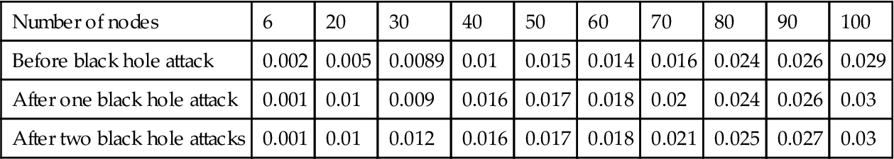
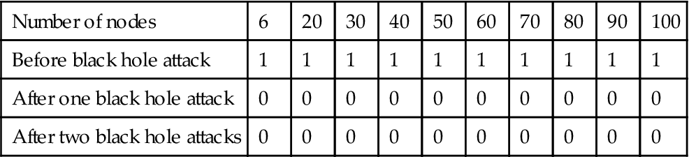
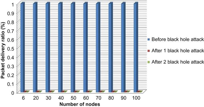
Table 4.4
Packet Delivery Ratio Comparison
| Number of nodes | 6 | 20 | 30 | 40 | 50 | 60 | 70 | 80 | 90 | 100 |
| Before black hole attack | 1 | 1 | 1 | 1 | 1 | 1 | 1 | 1 | 1 | 1 |
| After one black hole attack | 0 | 0 | 0 | 0 | 0 | 0 | 0 | 0 | 0 | 0 |
| After two black hole attacks | 0 | 0 | 0 | 0 | 0 | 0 | 0 | 0 | 0 | 0 |
As we can see from Table 4.1, total drop packets of the black hole AODV is exaggerated more than the conventional AODV network simulations in all situations. We perceive from Table 4.1 that the packet loss already exists within the network. Also this is a result of packet drop at the node interface queue as a result of the density of knowledge traffic. Thus, we tend to alter node and packet parameters to reduce the information traffic. Desperate to evaluate the black hole impact within the network, we have to reduce the packet loss that happens at the network, except the black hole. In an exceedingly wireless ad hoc network that does not have any black hole, the information traffic could be dense and packets would possibly get lost, for example, in FTP traffic. Therefore, the information loss does not continuously say there was a black hole node within the network.
In Fig. 4.17, which is drawn from above table data, we can compare total drop packets before black hole attack and after one and two black hole attacks:
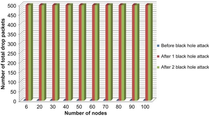
Table 4.2 shows average end-to-end delay in different scenarios, as we can see average end-to-end delay increase in scenarios with black hole attack, it is because of dropping packets after receiving packets by black hole nodes.
Fig. 4.18, which is drawn from above table’s data, compares end-to-end delay before black hole attack and after one and two black hole attacks:
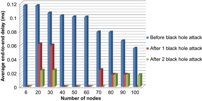
Table 4.3 shows routing request overhead for different scenarios. After entering black hole, nodes into the network routing request overhead increase; that means after black hole attack, number of data packets that transmit are less than number of control packets generate.
Fig. 4.19 is drawn from above table’s data, which can compare routing overhead before black hole attack and after one and two black hole attacks:
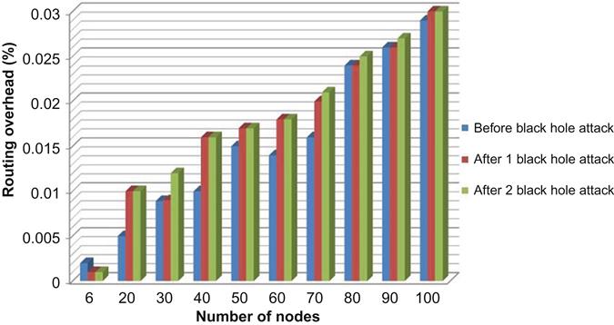
Table 4.4 compares packet delivery ratio (PDR). As it shows, PDR is almost 1 before black hole attack that it means almost total packets sent by sender node are received by receiver node, but for network with black hole node PDR reduces to 0, that means almost whole of the packets sent by sender node are dropped by black hole nodes.
Fig. 4.20 is drawn from above table’s data, which can compare PDR before black hole attack and after one and two black hole attacks:
4.5 Summary
This chapter investigated the performance of network before black hole attack, after single black hole attack, and after multiple black hole attacks. The output of this chapter is direct input for the next chapter. The purpose of this chapter is displaying network performance with single black hole attack and multiple black hole attacks and examining network performance under this attack.