
Embedded Multicore Software Development
Rob Oshana Vice President Software Engineering R&D, NXP Semiconductors, Austin, TX, United States
Abstract
A multicore processor is a computing device that contains two or more independent processing elements (referred to as cores) integrated on to a single device that read and execute program instructions. There are many architectural styles of multicore processors and many application areas such as embedded processing, graphics processing, and networking.
Keywords
Multicore; Heterogeneous; Homogeneous; Optimization; Parallelism; Scalability
A multicore processor is a computing device that contains two or more independent processing elements (referred to as cores) integrated on to a single device that read and execute program instructions. There are many architectural styles of multicore processors and many application areas such as embedded processing, graphics processing, and networking.
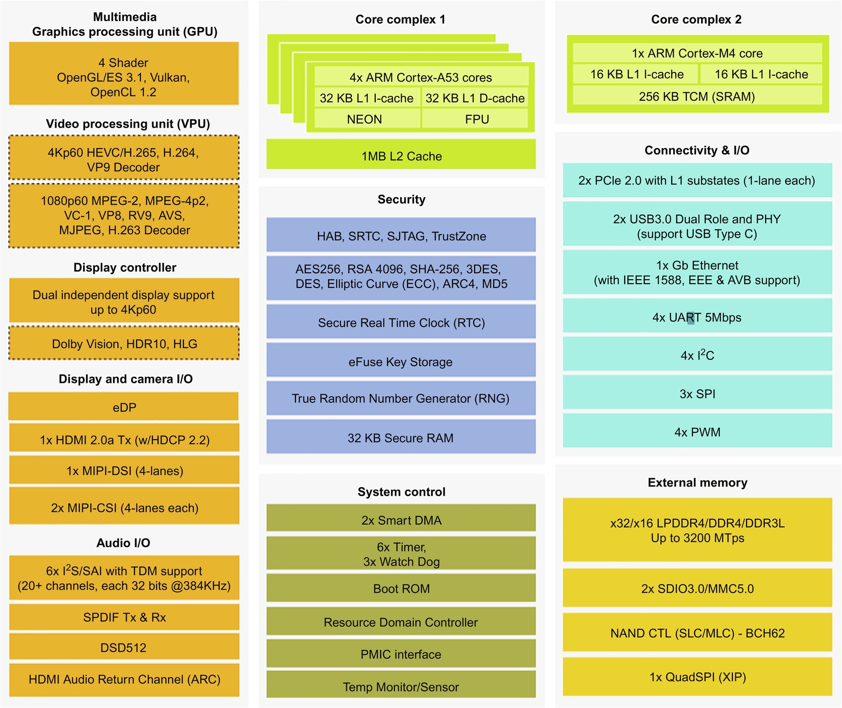
A typical multicore processor will have multiple cores that can be the same (homogeneous) or different (heterogeneous), accelerators (the more generic term is processing element) for dedicated functions such as video or network acceleration, and a number of shared resources (memory, cache, peripherals such as ethernet, display, codecs, and UART) (Fig. 1).
A key algorithm that should be memorized when thinking about multicore systems is the following:
- • Parallelism is all about exposing parallelism in the application.
- • Memory hierarchy is all about maximizing data locality in the network, disk, RAM, cache, core, etc.
- • Contention is all about minimizing interactions between cores (e.g., locking, synchronization, etc.).
To achieve the best performance we need to achieve the best possible parallelism, use memory efficiently, and reduce the contention. As we move forward we will touch on each of these areas.
1 Symmetric and Asymmetric Multiprocessing
Efficiently allocating resources in multicore systems can be a challenge. Depending on the configuration the multiple software components in these systems may or may not be aware of how other components are using these resources. There are two primary forms of multiprocessing (as shown in Fig. 2):
- • Symmetric multiprocessing
- • Asymmetric multiprocessing

1.1 Symmetric Multiprocessing
Symmetric multiprocessing (SMP) uses a single copy of the operating system on all the system’s cores. The operating system has visibility into all system elements and can allocate resources to multiple cores with little or no guidance from the application developer. SMP dynamically allocates resources to specific applications rather than to cores, which leads to greater utilization of available processing power. Key characteristics of SMP include:
- • A collection of homogeneous cores with a common view of system resources such as sharing a coherent memory space and using CPUs that communicate using a large coherent memory space.
- • Applicable for general-purpose applications or applications that may not be entirely known at design time. Applications that may need to suspend because of memory accesses, or may need to migrate or restart on any core, fit into an SMP model as well. Multithreaded applications are SMP friendly.
- • SMP is not as good for specific known tasks like data-intensive applications such as audio, video, or signal processing.
1.2 Asymmetric Multiprocessing
Asymmetric multiprocessing (AMP) can be:
- • homogeneous—each CPU runs the same type and version of the operating system; or
- • heterogeneous—each CPU runs either a different operating system or a different version of the same operating system.
In heterogeneous systems you must either implement a proprietary communications scheme or choose two OSs that share a common API and infrastructure for interprocessor communications. There must be well-defined and implemented methods for accessing shared resources.
In an AMP system an application process will always runs on the same CPU, even when other CPUs run idle. This can lead to one CPU being underutilized or overutilized. In some cases it may be possible to migrate a process dynamically from one CPU to another. There may be side effects of doing this such as requiring checkpointing of state information or a service interruption when the process is halted on one CPU and restarted on another CPU. This is further complicated if the CPUs run different operating systems.
In AMP systems the processor cores communicate using large coherent bus memories, shared local memories, hardware FIFOS, and other direct connections.
AMP is better applied to known data-intensive applications where it is better at maximizing efficiency for every task in the system such as audio and video processing. AMP is not as good as a pool of general computing resources.
The key reason there are AMP multicore devices is because they are the most economical way to deliver multiprocessing to specific tasks. The performance, energy, and area envelope is much better than SMP.
2 Parallelism Saves Power
Multicore reduces average power comsumption. It is becoming harder to achieve increased processor performance from traditional techniques such as increasing the clock frequency or developing new architectural approaches to increase instructions per cycle (IPC). Frequency scaling of CPU cores is no longer valid, primarily due to power challenges.
An electronic circuit has a capacitance C associated with it. Capacitance is the ability of a circuit to store energy. This can be defined as:
And the charge on a circuit can therefore be q = CV.
Work can be defined as the act of pushing something (charge) across a “distance.” In this discussion we can define this in electrostatic terms as pushing the charge from 0 to V volts in a circuit:
Power is defined as work over time, or in this discussion it is how many times a second we oscillate the circuit.
We can use an example to reflect this. Let us assume the circuit is as in Fig. 3.

This simple circuit has a capacitance C, a voltage V, a frequency F, and therefore a power defined as P = CV2F.
If we instead use a multicore circuit (as shown in Fig. 4) we can make the following assumptions:
- • We will use two cores instead of one.
- • We will clock this circuit as half the frequency for each of the two cores.
- • We will use more circuitry (capacitance C) with two cores instead of one, plus some additional circuitry to manage these cores, assume 2.1X the capacitance.
- • By reducing the frequency we can also reduce the voltage across the circuit. Let’s assume we can use a voltage of 0.7 or the single core circuit (it could be half the single core circuit but let’s assume a bit more for additional overhead).

Given these assumptions, power can be defined as:
What this says is by going from one core to multicore we can reduce overall power consumption by over 48%, given the conservative assumptions above.
There are other benefits from going to multicore. When we can use several smaller simpler cores instead of one big complicated core we can achieve more predictable performance and achieve a simpler programming model in some cases.
3 Look for Parallelism Opportunities
A computer program always has a sequential part and a parallel part. What does this mean? Let’s start with a simple example:
- 1. A = B + C
- 2. D = A + 2
- 3. E = D + A
- 4. For (i = 0; i < E; i ++)
- 5. N(i) = 0
In this example Steps 1, 2, and 4 are “sequential.” There is a data dependence that prevents these three instructions from executing in parallel.
Steps 4 and 5 are parallel. There is no data dependence and multiple iterations of N(i) can execute in parallel.
Even with E a large number—say, 200—the best we can do is to sequentially execute four instructions, no matter how many processors we have available to us.
When algorithms are implemented serially there is a well-defined operation order that can be very inflexible. In the edge detection example for a given data block the Sobel cannot be computed until after the smoothing function completes. For other sets of operations, such as within the correction function, the order in which pixels are corrected may be irrelevant.
Dependencies between data reads and writes determine the partial order of computation. There are three types of data dependencies that limit the ordering: true data dependencies, antidependencies, and output dependencies (Fig. 5).

True data dependencies imply an ordering between operations in which a data value may not be read until after its value has been written. These are fundamental dependencies in an algorithm, although it might be possible to refactor algorithms to minimize the impact of this data dependency.
Antidependencies have the opposite relationship and can possibly be resolved by variable renaming. In an antidependency a data value cannot be written until the previous data value has been read. In Fig. 5 the final assignment to A cannot occur before B is assigned because B needs the previous value of A. In the final assignment variable A is renamed to D, then the B and D assignments may be reordered.
Renaming may increase storage requirements when new variables are introduced if the lifetimes of the variables overlap as code is parallelized. Antidependencies are common occurrences in sequential code. For example, intermediate variables defined outside the loop may be used within each loop iteration. This is fine when operations occur sequentially. The same variable storage may be repeatedly reused. However, when using shared memory, if all iterations were run in parallel, they would be competing for the same shared intermediate variable space. One solution would be to have each iteration use its own local intermediate variables. Minimizing variable lifetimes through proper scoping helps to avoid these dependency types.
The third type of dependency is the output dependency. In an output dependency writes to a variable may not be reordered if they change the final value of the variable that remains when the instructions are complete. In the “output dependency” of Fig. 5 the final assignment to A may not be moved above the first assignment because the remaining value will not be correct.
Parallelizing an algorithm requires both honoring dependencies and appropriately matching the parallelism to the available resources. Algorithms with a high number of data dependencies will not parallelize effectively. When all antidependencies are removed and still partitioning does not yield acceptable performance, consider changing algorithms to find an equivalent result using an algorithm that is more amenable to parallelism. This may not be possible when implementing a standard with strictly prescribed algorithms. In other cases there may be effective ways to achieve similar results.
Let’s take a look at some examples:

Loop 1: a [0] = a [-1] + b [0]
Loop 2: a [1] = a [0] + b [1]
……
Loop N: a [N] = a [N-1] + b [N]
Here Loop 2 is dependent on the result of Loop 1: to compute a [1] one needs a [0], which can be obtained from Loop 1. Hence, Loop nest 1 cannot be parallelized because there is a loop-carried dependence flow on the other loop.

Loop 1: a [0] = a [0] + b [0]
Loop 2: a [1] = a [1] + b [1]
…….
Loop N: a [N] = a [N] + b [N]
Here Loop nest 2 can be parallelized because the antidependency from the read of an [i] to the write of an [i] has an (=) direction and it’s not loop carried.

Loop 1: a [0] = a [-1]
Loop 2: a [4] = a [1]
……
Loop N: a [4*N] = a [2*N-1]
We can see that there is no dependency between any loops in Loop nest 3. Hence Loop nest 3 can be parallelized.
Multicore architectures have sensitivity to the structure of software. In general, parallel execution incurs overhead that limits the expected execution time benefits that can be achieved. Performance improvements therefore depend on software algorithms and their implementations. In some cases parallel problems can achieve speedup factors close to the number of cores, or potentially more if the problem is split up to fit within each core’s cache(s), which avoids the use of the much slower main system memory. However, as we will show, many applications cannot be accelerated adequately unless the application developer spends a significant effort to refactor the portions of the application.
As an example, we can think of an application as having both sequential parts and parallel parts (as shown in Fig. 6).

This application, when executed on a single core processor, will execute sequentially and take a total of 12 time units to complete (Fig. 7).

If we run this same application on a dual-core processor (Fig. 8), the application will take a total of 7 time units, limited by the sequential part of the code that cannot execute in parallel due to reasons we showed earlier.

This is a speedup of 12/7 = 1.7X from the single-core processor.
If we take this further to a four-core system (Fig. 9), we can see a total execution time of 5 units for a total speedup of 12/5 = 2.4X from the single-core processor and 7/5 = 1.4X over the two-core system.
If the fraction of the computation that cannot be divided into concurrent tasks is f and no overhead incurs when the computation is divided into concurrent parts, the time to perform the computation with n processors is given by tp ≥ fts + [(1 − f)ts]/n (as shown in Fig. 10).

The general solution to this is called Amdahl’s Law and is shown in Fig. 11.

Amdahl’s Law states that parallel performance is limited by the portion of serial code in the algorithm. Specifically:
where S is the portion of the algorithm running serialized code, and N is the number of processors running parallelized code.
Amdahl’s Law implies that adding additional cores results in additional overheads and latencies. These overheads and latencies serialize execution between communicating and noncommunicating cores by requiring the use of mechanisms such as hardware barriers and resource contention. There are also various interdependent sources of latency and overhead due to processor architecture (e.g., cache coherency), system latencies and overhead (e.g., processor scheduling), and application latencies and overhead (e.g., synchronization).
Parallelism overhead comes from areas such as:
- • Overhead from starting a thread or process.
- • Overhead of communicating shared data.
- • Overhead of synchronizing.
- • Overhead from extra (redundant) computation required to parallelize some parallel algorithms.
Of course Amdahl’s Law is sensitive to application workloads (e.g., data dependencies) and predicts that as the number of cores increase so do the size of the overheads and latencies as well.
Let’s look at a couple more quick examples.
Assume 95% of a program’s execution time occurs inside a loop that can be executed in parallel. What is the maximum speedup we should expect from a parallel version of the program executing on eight CPUs?

where S is the portion of the algorithm running serialized code, N is the number of processors running serialized code, 95% of the program’s execution time can be executed in parallel, eight CPUs, S = 1 − 0.95 = 0.05, and N = 8:

where speedup = 5.9.
Assume 5% of a parallel program’s execution time is spent within inherently sequential code. What is the maximum speedup achievable by this program, regardless of how many processing elements are used?
where 5% parallel program’s execution time is spent within inherently sequential code, and N = ∞:

3.1 Multicore Processing Granularity
Granularity can be described as the ratio of computation to communication in a parallel program. There are two types of granularity (as shown in Fig. 12).

Fine-grained parallelism implies partitioning the application into small amounts of work leading to a low computation-to-communication ratio. For example, if we partition a “for” loop into independent parallel computions by unrolling the loop, this would be an example of fine-grained parallelism. One of the downsides to fine-grained parallelism is that there may be many synchronization points—for example, the compiler will insert synchronization points after each loop iteration, which may cause additional overhead. Moreover, many loop iterations would have to be parallelized to get decent speedup, but there the developer has more control over load-balancing the application.
Coarse-grained parallelism is where there is a high computation-to-communication ratio. For example, if we partition an application into several high-level tasks that then get allocated to different cores, this would be an example of coarse-grained parallelism. The advantage of this is that there is more parallel code running at any point in time and fewer synchronizations are required. However, load-balancing may not be ideal as the higher level tasks are usually not all equivalent as far as execution time is concerned.
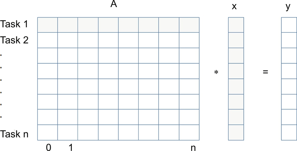
Let’s take one more example. Let’s say we want to multiply each element of an array A by a vector X (Fig. 13). Let’s think about how to decompose this problem into the right level of granularity. The code for something like this would look like:

for (i = 0, N-1)
 for (j = 0, N-1)
   y[i] = A[i,j] * x[j];
From this algorithm we can see that each output element of y depends on one row of A and all of x. All tasks are of the same size in terms of number of operations.
How can we break this into tasks? Course grained with a smaller number of tasks or fine grained with a larger number of tasks. Fig. 14 shows an example of each.

4 Multicore Application Locality
As you may know from your introductory computer architecture courses in college large memories are slow and fast memories are small (Fig. 15). The slow accesses to “remote” data we can generalize as “communication.”
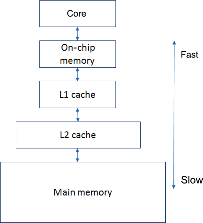
In general, storage hierarchies are large and fast. Most multicore processors have large, fast caches. Of course, our multicore algorithms should do most work on local data closer to the core.
Let’s first discuss how data are accessed. To improve performance in a multicore system (or any system for that matter) we should strive for these two goals:
- 1. Data reuse—when possible reuse the same or nearby data multiple times. This approach is mainly intrinsic in computation.
- 2. Data locality—with this approach the goal is for data to be reused and present in “fast memory” like a cache. Take advantage of the same data or the same data transfer.
Computations that have reuse can achieve locality using appropriate data placement and layout as well as intelligent code reordering and transformations.
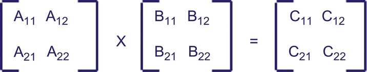
Let’s take the example of a matrix multiply. We will consider a “naive” version of matrix multiply and a “cache” version. The “naive” version is the simple, triply-nested implementation we are typically taught in school. The “cache” version is a more efficient implementation that takes the memory hierarchy into account. A typical matrix multiply is shown in Fig. 16.

One consideration with matrix multiplication is that the row-major versus column-major storage pattern is language dependent.
Languages like C and C ++ use a row-major storage pattern for two-dimensional matrices. In C/C ++ the last index in a multidimensional array indexes contiguous memory locations. In other words, a[i][j] and a[i][j + 1] are adjacent in memory (see Fig. 17).

The stride between adjacent elements in the same row is 1. The stride between adjacent elements in the same column is the row length (10 in the example in Fig. 21).
This is important because memory access patterns can have a noticeable impact on performance, especially on systems with a complicated multilevel memory hierarchy. The code segments in Fig. 18 access the same elements of an array, but the order of accesses is different.

We can apply additional optimizations including “blocking.” “Block” in this discussion does not mean “cache block.” Instead, it means a subblock within the matrix we are using in this example.
As an example of a “block” we can break our matrix into blocks (N = 8; subblock size = 4):
Here is the way it works—instead of the row access model that we just described:
/* row access method */
for (i = 0; i < N; i = i + 1)
for (j = 0; j < N; j = j + 1)
   {r = 0;
   for (k = 0; k < N; k = k + 1){
    r = r + y[i][k]*z[k][j];};
   x[i][j] = r;
   };
With the blocking approach we use two inner loops. One loop reads all the N × N elements of z[]. The other loop will read N elements of one row of y[] repeatedly. The final step is to write N elements of one row of x[].
Subblocks (i.e., Axy) can be treated just like scalars in this example and we can compute:
- C11 = A11B11 + A12B21
- C12 = A11B12 + A12B22
- C21 = A21B11 + A22B21
- C22 = A21B12 + A22B22
Now a “blocked” matrix multiply can be implemented as:
for (jj = 0; jj < n; jj +=bsize) {
 for (i = 0; i < n; i ++)
 for (j = jj; j < min(jj + bsize,n); j ++)
 c[i][j] = 0.0;
 for (kk = 0; kk < n; kk +=bsize) {
 for (i = 0; i < n; i ++) {
 for (j = jj; j < min(jj + bsize,n); j ++) {
 sum = 0.0
 for (k = kk; k < min(kk + bsize,n); k ++) {
 sum += a[i][k] * b[k][j];
 }
 c[i][j] += sum;
 }
 }
 }
}
In this example the loop ordering is bijk. The innermost loop pair multiplies a 1 X b-size sliver of A by a b-size X b-size block of B and sums into a 1 X b-size sliver of C. We then loop over i steps through n row slivers of A and C, using the same B (see Fig. 19).

The results are shown in Fig. 20A. As you can see, row order access is faster than column order access.

Of course, we can also increase the number of threads to achieve higher performance (as shown in Fig. 25 as well). Since this multicore processor has only four cores, running with more than four threads—when threads are computer bound—this only causes the OS to “thrash” as it switches threads across the cores. At some point you can expect the overhead of too many threads to hurt performance and slow an application down. See the discussion on Amdahl’s Law a little earlier!
The importance of efficient caching for multicore performance cannot be overstated.
You need not only to expose parallelism, but also to take into account the memory hierarchy and work hard to eliminate/minimize contention. This becomes increasingly true because as the number of cores grows so does the contention between cores.
4.1 Load Imbalance
Load imbalance is the time that processors in the system are idle due to (Fig. 21):
- • Insufficient parallelism (during that phase).
- • Unequal size tasks.

Unequal size tasks can include things like tree-structured computations and other fundamentally unstructured problems. The algorithm needs to balance load where possible and the developer should profile the application on the multicore processor to look for load-balancing issues. Resources can sit idle when load-balancing issues are present.
4.2 Data Parallelism
Data parallelism is a parallelism approach in which multiple units process data concurrently. Performance improvement depends on many cores being able to work on the data at the same time. When the algorithm is sequential in nature, difficulties arise. For example, cryptoprotocols, such as 3DES (triple data encryption standard) and AES (advanced encryption standard) are sequential in nature and therefore difficult to parallelize. Matrix operations are easier to parallelize because data are interlinked to a lesser degree (we have an example of this coming up).
In general, it is not possible to automate data parallelism in hardware or with a compiler because a reliable, robust algorithm is difficult to assemble to perform this in an automated way. The developer has to own part of this process.
Data parallelism represents any kind of parallelism that grows with the data set size. In this model the more data you give to the algorithm, the more tasks you can have and operations on data may be the same or different. But the key to this approach is its scalability.
Fig. 22 shows the scalable nature of data parallelism.

In the example given in Fig. 23 an image is decomposed into sections or “chunks” and partitioned to multiple cores to process in parallel. The “image in” and “image out” management tasks are usually performed by one of the cores (an upcoming case study will go into this in more detail).

4.3 Task Parallelism
Task parallelism distributes different applications, processes, or threads to different units. This can be done either manually or with the help of the operating system. The challenge with task parallelism is how to divide the application into multiple threads. For systems with many small units, such as a computer game, this can be straightforward. However, when there is only one heavy and well-integrated task the partitioning process can be more difficult and often faces the same problems associated with data parallelism.
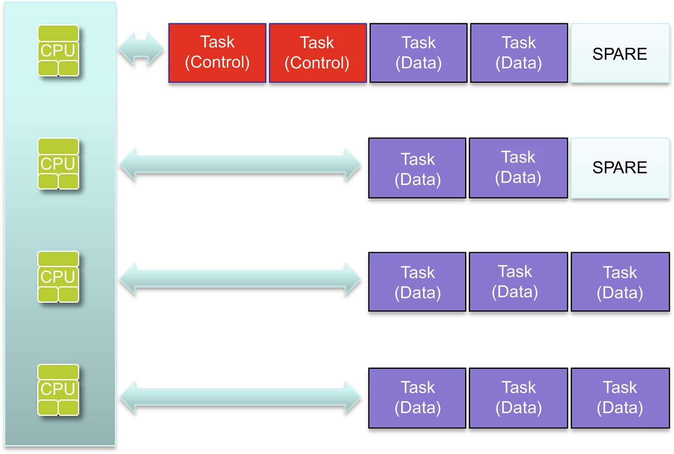
Fig. 24 is an example of task parallelism. Instead of partitioning data to different cores the same data are processed by each core (task), but each task is doing something different on the data.

Task parallelism is about functional decomposition. The goal is to assign tasks to distinct functions in the program. This can only scale to a constant factor. Each functional task, however, can also be data parallel. Fig. 25 shows this. Each of these functions (atmospheric, ocean, data fusion, surface, wind) can be allocated to a dedicated core, but only the scalability is constant.

5 Multicore Programming Models
A “programming model” defines the languages and libraries that create an abstract view of a machine. For multicore programming the programming model should consider the following:
- • Control—this part of the programming model defines how parallelism is created and how dependencies (orderings) are enforced. An example of this would be to define the explicit number of threads of execution.
- • Data—this part of the programming model defines how and whether data can be shared or kept private. For shared data this also defines whether the data are shared data accessed or private data communicated. For example, what is the access to global data from multiple threads? What is the control of data distribution to execution threads?
- • Synchronization—this part of the programming model defines which operations can be used to coordinate parallelism and which are atomic (indivisible) operations. An example of this is communication (e.g., which data transfer parts of the language will be used or which libraries are used). Another example would be to define explicitly the mechanisms to regulate access to data. Fig. 26 is an example of a programming model decision between threading (shared memory) and message passing. As we will soon see this drives decisions on which technology to use in multicore development.

Fig. 26 Multicore programming model decision (threading use of shared memory or message passing).
The shared memory paradigm in some ways is similar to sequence programming, but the developer must explicitly specify parallelism and use some mechanism (locks/semaphors) to control access to the shared memory. Sometimes this is called directive based and we can use technologies like OpenMP to help us with this.
The choice is explicit from a parallel-programming perspective. We can use pthreads that are common to a shared memory system and focus on synchronization, or we can use a technology like Message Passing Interface (MPI), which is based on message-passing systems where the focus is on communication—not so much synchronization.
Determining the right programming model for a multicore system is dependent on several factors:
- • The type of multicore processor—different multicore processors support different types of parallelism and programming.
- • The level of abstraction required—from “do it yourself” (DIY) multicore to using abstraction layers.
6 Performance and Optimization of Multicore Systems
In this section we will discuss optimization techniques for multicore applications. But, before we begin, let’s start with a quote. Donald Knuth has said:
Programmers waste enormous amounts of time thinking about, or worrying about, the speed of noncritical parts of their programs, and these attempts at efficiency actually have a strong negative impact when debugging and maintenance are considered. We should forget about small efficiencies, say about 97% of the time: premature optimization is the root of all evil.
Indeed, premature optimization as well as excessive optimization (not knowing when to stop) are harmful in many ways. Discipline and an iterative approach are key to effective performance tuning. The Multicore Programming Practice Guide, like many other sources of performance tuning, has its recommendation for performance tuning of multicore applications (as shown in Fig. 27).

Let’s look at the top performance tuning and acceleration opportunities for multicore applications. We will focus on software-related optimizations, but also discuss some hardware approaches as well since they ultimately are related to software optimizations. The list we will discuss is:
- 1. Select the right “core” for your multicore
- 2. Improve serial performance before migrating to multicore
- 3. Achieve proper load balancing (SMP Linux)
- 4. Improve data locality
- 5. Reduce or eliminate false sharing
- 6. Use affinity scheduling when necessary
- 7. Apply the proper lock granularity and frequency
- 8. Remove sync barriers where possible
- 9. Minimize communication latencies
- 10. Use thread pools
- 11. Manage thread count
- 12. Stay out of the kernel if at all possible
- 13. Use parallel libraries (pthreads, openMP, etc.)
Let’s explore these one by one.
6.1 Select the Right “Core” for Your Multicore
Do you need a latency-oriented core or a throughput-oriented core? Do you need hardware acceleration or not? Is a heterogeneous architecture needed or a homogeneous one? It makes a big difference from a performance perspective. I put this in this section as well because it makes software programming more efficient without having to resort to fancy tips and tricks to get decent performance. But it does require benchmarking and analysis of the core and software development tools such as the compiler and the operating system.
6.2 Improve Serial Performance Before Migrating to Multicore (Especially Instruction-Level Parallelism)
Early in the development process, before looking at optimizations specific to multicore, it’s necessary to spend time improving the serial (single-core) application performance. Sequential execution must first be efficient before moving to parallelism to achieve higher performance. Early sequential optimization is much easier and less time consuming and less likely to introduce bugs.
Many performance improvements obtained in serial implementation will close the gap on the parallelism required to achieve your goals when moving to multicore. It’s much easier to focus on parallel execution alone during this migration, instead of having to worry about both sequential and parallel optimization at the same time.
Just be careful not to introduce serial optimizations that degrade or limit parallelism (such as unnecessary data dependencies) or overexploiting details of the single-core hardware architecture (such as cache capacity).
Focus on instruction-level parallelism (ILP). The compiler can help. The main goal of a compiler is to maintain the functionality of the application and support special functionality provided by the target and the application such as pragmas, instrinsics, and other capability like OpenMP, which we will discuss further. For example, the “restrict” keyword (C99 standard of the C programming language) is used in pointer declarations, basically telling the compiler that for the lifetime of the pointer only it or a value derived from it (such as pointer + 1) can be used to access an object it points to. This limits the effects of memory disambiguation or pointer aliasing, which enables more aggressive optimizations. An example of this is given below. In this example stores may alias loads. This forces operations to be executed sequentially:
void VectorAddition(int *a, int *b, int *c)
{
 for (int i = 0; i < 100; i ++)
   a[i] = b[i] + c[i];
}
In this example the “restrict” keyword allows independent loads and stores. Operations can now be performed in parallel:
void VectorAddition(int restrict a, int *b, int *c)
{
 for (int i = 0; i < 100; i ++)
   a[i] = b[i] + c[i];
}
The “restrict” keyword can enable more aggressive optimizations such as software pipelining. Software pipelining is a powerful loop optimization usually performed by the compiler back end. It consists of scheduling instructions across several iterations of a loop. This optimization (Fig. 28) enables instruction-level parallelism, reduces pipeline stalls, and fills delay slots. Loop iterations are scheduled so that an iteration starts before the previous iteration has completed. This approach can be combined with loop unrolling (see below) to achieve significant efficiency improvements.

Loop transformations also enable ILP. Loops are typically the hotspots of many applications. Loop transformations are used to organize the sequence of computations and memory accesses to better fit the processor internal structure and enable ILP.
One example of a loop transformation to enable ILP is called loop unrolling. This transformation can decrease the number of memory accesses and improve ILP. It unrolls the outer loop inside the inner loop and increases the number of independent operations inside the loop body.
Below is an example of a doubly nested loop:
for (i = 0; i < N; i +++)
{
 for (j = 0; j < N; j ++)
 {
   a[i][j] = b[j][i];
 }
}
Here is the same loop with the loop unrolled, enabling more ILP:
for (i = 0; i < N; i +++)
{
 for (j = 0; j < N; j ++)
 {
   a[i][j] = b[j][i];
   a[i + 1][j] = b[j][i + 1];
 }
}
This approach improves the spatial locality of b and increases the size of loop body and therefore the available ILP. Loop unrolling also enables more aggressive optimizations such as vectorizations (SIMD) by allowing the compiler to use these special instructions to improve performance even more (as shown in Fig. 29 where the “move.4w” instructions are essentially SIMD instructions operating on four words of data in parallel).

As with all optimizations you need to use the right ones for the application. Take the example of video versus audio algorithms. For example, audio applications are based on a continuous feed of data samples. There are lots of long loops to process. This is a good application structure to use software pipelining, which works well in this situation.
Video applications, on the other hand, are designed to break up video frames into smaller blocks (like the example earlier, we called this minimal coded units, MCUs). This type of structure uses small loop counts and many blocks of processing. Software pipelining in this case is not as efficient due to the long prologs required for pipelining. There is too much overhead for each loop. In this case it’s best to use loop unrolling instead, which works better and more efficiently for these smaller loops.
There are many other examples of sequential optimization. The key message is to make sure you apply these first before worrying about other parallel optimizations.
6.3 Achieve Proper Load Balancing (SMP Linux) and Scheduling
Multicore-aware operating systems like Linux have infrastructure to support multicore performance at the system level such as SMP schedulers, different forms of synchronization, load-balancers for interrupts, affinity-scheduling techniques and CPU isolation. If used properly, overall system performance can be optimized. However, they all have some inherent overhead so they must be used properly.
Linux is a multitasking kernel that allows more than one process to exist at any given time. The Linux process scheduler manages which process runs at any given time. The basic responsibilities are:
- • Share the cores equally among all currently running processes.
- • Select the appropriate process to run next (if required), using scheduling and process priorities.
- • Rebalance processes between multiple cores in SMP systems if necessary.
Multicore applications are generally categorized to be either CPU bound or I/O bound. CPU-bound applications spend a lot of time using the CPU to do computations (like server applications). I/O-bound applications spend a lot of time waiting for relatively slow I/O operations to complete (e.g., like a smartphone waiting for user input, network accesses, etc.). There is obviously a trade-off here. If we let our task run for longer periods of time, it can accomplish more work but responsiveness (to I/O) suffers. If the time period for the task gets shorter, our system can react faster to I/O events. But now more time is spent running the scheduling algorithm between task switches. This leads to more overhead and efficiency suffers.
6.4 Improve Data Locality
Although this was discussed earlier, there are some additional comments to be made concerning software optimizations related to data locality. This is a key focus area for multicore optimization. In many applications this requires some careful analysis of the application. For example, let’s consider a networking application that is using the Linux operating system.
In the Linux operating system all network-related queues and buffers use a common data structure called sk_buff. This is a large data structure that holds all the control information needed for a network packet. sk_buff structure elements are organized as a doubly linked list. This allows efficient movement of sk_buff elements from the beginning/end of a list to the beginning/end of another list.
The standard sk_buff has information spread over three or more cache lines. Data-plane applications require only one cache line’s worth of information.
We can take advantage of this by creating a new structure that packs/aligns to a single cache line. If we are smart and make this part of the packet buffer headroom, then we don’t have to worry about cache misses and flushes each time we access the large sk_buff structure. Instead we use a small portion of this that fits neatly into the cache, improving data locality and efficiency. This is shown in Fig. 30.

6.5 Reduce or Eliminate False Sharing
False sharing occurs when two software threads manipulate data that are on the same cache line. As we discussed earlier the memory system of a multicore processor must ensure cache coherency in SMP systems. Any modifications made to shared cache must be flagged to the memory system so each processor is aware the cache has been modified. The affected cache line is “invalidated” when one thread has changed data on that line of cache. When this happens the second thread must wait for the cache line to be reloaded from memory (Fig. 31).

The code below shows this condition. In this example sum_temp1 may need to continually reread “a” from main memory (instead of from cache) even though inc_b’s modification of “b” should be irrelevant.
In this situation if the extra prefetched words are not needed and another processor in this cache-coherent, shared memory system must immediately change these words, this extra transfer has a negative impact on system performance and energy consumption:
struct data
{
  volatile int a;
  volatile int b;
};

data f;

int sum_temp1()
{
  int s = 0;
  for (int i = 0; i < 1000; i ++)
 s += f.a;
  return s;
}

void inc_b()
{
  for (int i = 0; i < 1000; i ++)
 ++f.b;
}
One solution to this condition is to pad the data in the data structure so that the elements causing false-sharing performance degradation will be allocated to different cache lines:

6.6 Use Affinity Scheduling When Necessary
In some applications it might make sense to force a thread to continue executing on a particular core instead of letting the operating system make the decision whether or not to move the thread to another core. This is referred to as “processor affinity.” Operating systems like Linux have APIs to allow a developer to control this, allowing them the ability to map certain threads to cores in a multicore processor (Fig. 32).

On many processor architectures any migration of threads across cache, memory, or processor boundaries can be expensive (flushing the cache, etc.). The developer can use APIs to set the affinities for certain threads to take advantage of shared caches, interrupt handing, and to match computation with data (locality). A snippet of code that shows how to do this is:
#define _GNU_SOURCE
#include < sched.h >
long
sched_setaffinity(pid_t pid, unsigned int len,
     unsigned long *user_mask_ptr);
long
sched_getaffinity(pid_t pid, unsigned int len,
     unsigned long *user_mask_ptr);
In this code snippet the first system call will set the affinity of a process. The second system call retrieves the affinity of a process.
The PID argument is the process ID of the process you want to set or retrieve. The second argument is the length of the affinity bitmask. The third argument is a pointer to the bitmask. Masks can be used to set the affinity of the cores of interest.
If you set the affinity to a single CPU this will exclude other threads from using that CPU. This also takes that processor out of the pool of resources that the OS can allocate. Be careful every time you are manually controlling affinity scheduling. There may be side effects that are not obvious. Design the affinity-scheduling scheme carefully to ensure efficiency.
6.7 Apply the Proper Lock Granularity and Frequency
There are two basic laws of concurrent execution:
- 1. The program should not malfunction.
- 2. Concurrent execution should not be slower than serial execution.
We use locks as a mutual exclusion mechanism to prevent multiple threads getting simultaneous access to shared data or code sections. These locks are usually implemented using semaphores or mutexes, which are essentially expensive API calls into the operating system.
Locks can be fine grained or coarse grained. Too many locks increases the amount of time spent in the operating system and increases the risk of deadlock. Coarse-grained locking reduces the chance of deadlock, but can cause additional performance degradations due to locking large areas of the application (mainly system latency).
Avoiding heavy use of locks and semaphores due to performance penalties. Here are some guidelines:
- • Organize global data structures into buckets and use a separate lock for each bucket.
- • Design the system to allow threads to compute private copies of a value and then synchronize only to produce the global result. This will require less locking.
- • Avoid spinning on shared variables waiting for events.
- • Use atomic memory read/writes to replace locks if the architecture supports this.
- • Avoiding atomic sections when possible (an atomic section is a set of consecutive statements that can only be run by one thread at a time).
- • Place locks only around commonly used fields and not entire structures if this is possible.
- • Compute all possible precalculations and postcalculations outside the critical section, as this will minimize the time spent in a critical section.
- • Make sure that locks are taken in the same order to prevent deadlock situations.
- • Use mechanisms that are designed to reduce overhead in the operating system. For example, in POSIX-based systems use the trylock() function that allows the program to continue execution to handle an unsuccessful lock. In Linux use the “futex” (fast user space mutex) to do resource checks in user space instead of the kernel (see Fig. 33).

Fig. 33 Locks versus barriers.
6.8 Remove Sync Barriers Where Possible
A synchronization barrier causes a thread to wait until the other threads have reached the barrier and is used to ensure that variables needed at a given execution point are ready to be used. It differs from a lock for this very reason (Fig. 33).
Barriers can have the same performance problem as locks if not used properly. Oversynchronizing can negatively impact performance. This is the reason barriers should only be used to ensure that data dependencies are respected and/or where the execution frequency is the lowest.
A barrier can be used to replace creating and destroying threads multiple times when dealing with a sequence of tasks (i.e., replacing join and create threads). Hence when used in this way certain performance improvements can be realized.
6.9 Minimize Communication Latencies
When possible limit communication in multicore systems. Even extra computing is often more efficient than communication in many cases. For example, one approach to minimize communication latencies is to distribute data by giving each CPU has its own local data set that it can work on. This is called per-cpu data and is a technique used in the Linux kernel for several critical subsystems. For example, the kernel slab allocator uses per-cpu data for fast CPU local memory allocation. The disadvantage is higher memory overhead and increased complexity dealing with CPU hotplug.
In general, the communication time can be estimated using the following:
where n is the size of the message, α is the startup time due to the latency, and β is the time for sending one data unit limited by the available bandwidth.
Here are a few other tips and tricks to reduce communication latency:
- • Gather small messages into larger ones when possible to increase the effective communications bandwidth (reduce β, reduce α, increase n).
- • Sending noncontiguous data is usually less efficient than sending contiguous data (increases α, decreases n).
- • Do not use messages that are too large. Some communication protocols change when messages get too large (increases α, increases n, increases β).
- • The layout of processes/threads on cores may affect performance due to communication network latency and the routing strategy (increases α).
- • Use asynchronous communication techniques to overlap communication and computation. Asynchronous communication (nonblocking) primitives do not require the sender and receiver to “rendezvous” (decrease α).
- • Avoid memory copies for large messages by using zero-copy protocols (decrease β).
6.10 Use Thread Pools
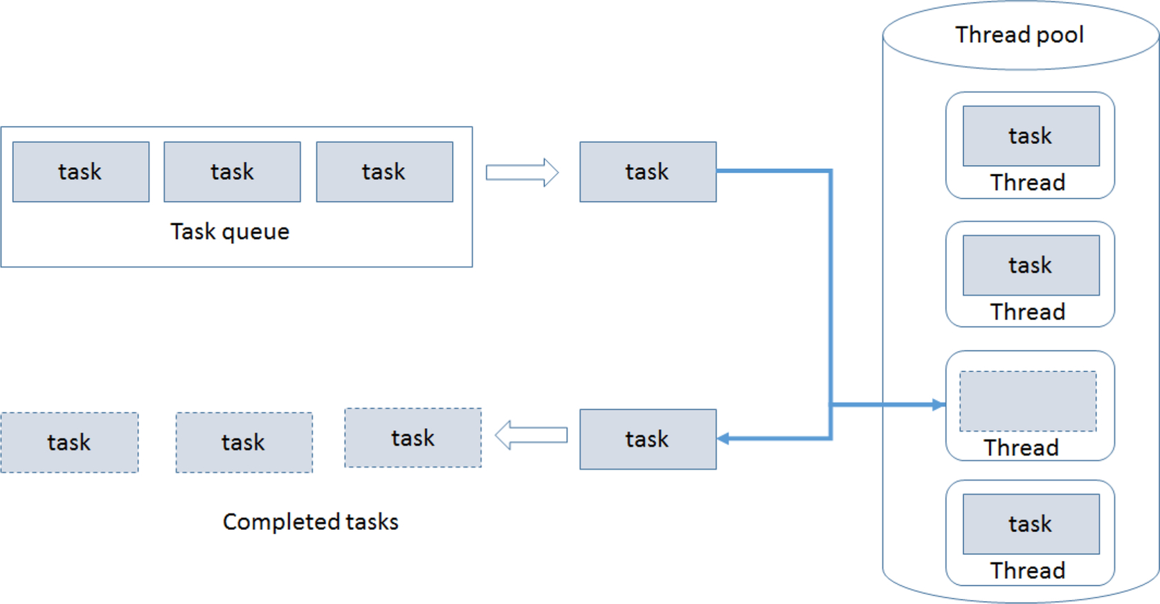
When using a peer or master/worker design, like the one we discussed earlier, users should not create new threads on the fly. This causes overhead. Instead have them stopped when they are not being used. Creating and freeing processes and threads is expensive. The penalty caused by the associated overhead may be larger than the benefit of running the work in parallel.
In this approach a number of threads are allocated to a thread pool. N threads are created to perform a number of operations M, where N ≪ M. When a threads completes the task it’s working on, it will then request the next task from the thread pool (usually organized into a queue) until all the tasks have been completed. The thread can then terminate (or sleep) until new tasks become available. Fig. 34 is a conceptual diagram of this.
A thread pool is implemented as a data structure as:
typedef struct _threadpool{
 int num_threads;    //number of active threads
 int qsize;    //queue size
 pthread_t *threads;    //pointer to threads
 work_t* qhead;    //queue head pointer
 work_t* qtail;    //queue tail pointer
 pthread_mutex_t qlock;   //lock on the queue list
 pthread_cond_t q_not_empty; //nonempty and empty condition vairiables
 pthread_cond_t q_empty;
 int shutdown;
 int dont_accept;
} thread_pool;
The associated C code can be implemented to control access to the thread pool’s data structure. This is not shown here, but there are plenty of examples you can find that show reference implementations.
6.11 Manage Thread Count
As discussed earlier, parallel execution always incurs some overhead resulting from functions such as task startup time, intertask synchronization, data communications, hardware bookkeeping (e.g., memory consistency), software overhead (libraries, tools, runtime system, etc.), and task termination time.
As a general rule, small tasks (fine grain) are usually inefficient due to the overhead to manage many small tasks. Large tasks could lead to load imbalance. In many applications there is a trade-off between having enough tasks to keep all cores busy and having enough computation in each task to amortize the overhead.
The optimal thread count can also be determined by estimating the average blocking time of the threads running on each core:
6.12 Stay Out of the Kernel If at All Possible
We gain a lot of support from operating systems, but when optimizing for performance it’s sometimes better to not go in and out of the operating system often, as this incurs overhead. There are many tips and tricks for doing this, so study the manual for the operating system and learn about the techniques available to optimize performance. For example, Linux supports SMP multicore using mechanisms like “futex” (fast user space mutex).
A futex is comprised of two components:
- • A kernelspace wait queue.
- • An integer in userspace.
In multicore applications the multiple processes or threads operate on the integer in userspace and only use expensive system calls when there is a need to request operations on the wait queue (Fig. 35). This would occur if there was a need to wake up waiting processes, or put the current process in the wait queue. Futex operations do not use system calls except when the lock is contended. However, since most operations do not require arbitration between processes this will not happen in most cases (Fig. 36).


6.13 Use Concurrency Abstractions (Pthreads, OpenMP, etc.)
For larger multicore applications, attempting to implement the entire application using threads is going to be difficult and time consuming. An alternative is to program atop a concurrency platform. Concurrency platforms are abstraction layers of software that coordinate, schedule, and manage multicore resources. Using concurrency platforms, such as OpenMP, thread-building libraries, and OpenCL, can not only speed time to market but also help with system-level performance. It may seem counterintuitive to use abstraction layers to increase performance. But these concurrency platforms provide frameworks that prevent the developer from making mistakes that could lead to performance problems.
Writing code for multicore can be tedious and time consuming. Here is an example showing the sequential code for a dot product:
#define SIZE 1000
Main() {
 double a[SIZE], b[SIZE];
 // Compute a and b
 double sum = 0.0;
 for(int i = 0, i < SIZE; i ++)
   sum += a[i] * b[i];
 // use sum….
}
Now let’s implement this same dot product using pthreads for a four-core multicore processor. Here is the code:
#include < iostream >
#include < pthread.h >
#define THREADS 4
#define SIZE 1000
using namespace std;
double a[SIZE], b[SIZE], sum;
pthread_mutex mutex_sum;
void *dotprod(void *arg) {
 int my_id = (int)arg;
 int my_first = my_id * SIZE/THREADS;
 int my_last = (my_id + 1) * SIZE/THREADS;
 double partial_sum = 0;
 for(int i = my_first; i < my_last && i < SIZE; i ++)
   partial_sum += a[i] * b[i];
 pthread_nmutex_lock(&mutex_sum);
 sum += partial_sum;
pthread_mutex_unlock(&mutex_sum);
pthread_exit((void*)0);
}
int main(int argc, char *argv[]) {
// compute a and b…
pthread_attr_t attr;
pthread_t threads[THREADS];
pthread_mutex_init(&mutex_sum, NULL);
pthread_attr_init(&attr);
pthread_attr_setdetachstate(&attr, PTHREAD_CREATE_JOINABLE);
sum = 0;
for(int i = 0; i < THREADS; i ++)
pthread_create(&threads[i], &attr, dotprod, (void*)i);
 pthread_attr_destroy(&attr);
 int status;
 for(int i = 0, i < THREADS; i ++)
   pthread_join(threads[i], (void**)&status);
 // use sum….
 pthread_mutex_destroy(&mutex_sum);
 pthread_exit(NULL);
}
As you can see, this implementation, although probably much faster on a multicore processor, is rather tedious and difficult to implement correctly. This do-it-yourself approach can definitely work, but there are abstractions that can be used to make this process easier. That is what this section is all about.
Multicore programming can be made easier using concurrency abstractions. These include but are not limited to:
- • Language extensions
- • Frameworks
- • Libraries
There exists a wide variety of frameworks, language extensions, and libraries. Many of these are built upon pthreads technology. Pthreads is the API of POSIX-compliant operating systems, like Linux, used in many multicore applications.
Let’s take a look at some of the different approaches to provide levels of multicore programming abstraction.
7 Language Extensions Example—OpenMP
OpenMP is an example of language extensions. It’s actually an API that must be supported by the compiler. OpenMP uses multithreading as the method of parallelizing, in which a master thread forks a number of slave threads and the task is divided among these threads. The forked threads run concurrently on a runtime environment that allocates threads to different processor cores.
This requires application developer support. Each section of code that is a candidate to run in parallel must be marked with a preprocessor directive. This is an indicator to the compiler to insert instructions into the code to form threads before the indicated section is executed. Upon completion of the execution of the parallelized code the threads join back into the master thread, and the application then continues in sequential mode again. This is shown in Fig. 37.

Each thread executes the parallelized section of code independently. There exist various work-sharing constructs that can be used to divide a task among the threads so that each thread executes its allocated part of the code. Both task parallelism and data parallelism can be achieved this way. The example code below shows an example of how code can be instrumented to achieve this parallelism. The execution graph is shown in Fig. 38.

Using basic OpenMP programming constructs can lead you toward realizing Amdahl’s Law by parallelizing those parts of a program that the application developer has identified to be concurrent and leaving the serial portions unaffected (Fig. 39).

OpenMP programs start with an initial master thread operating in a sequential region. When a parallel region is encountered (indicated by the compiler directive “#pragma omp parallel” in Fig. 40) new threads called worker threads are created by the runtime scheduler. These threads execute simultaneously on the block of parallel code. When the parallel region ends the program waits for all threads to terminate (called a join), and then resumes its single-threaded execution for the next sequential region.

The OpenMP specification supports several important programming constructs:
- 1. Support of parallel regions
- 2. Worksharing across processing elements
- 3. Support of different data environments (shared, private, …)
- 4. Support of synchronization concepts (barrier, flush, …)
- 5. Runtime functions/environment variables
We will not go into the details of all the APIs and programming constructs for OpenMP, but there are a few items to keep in mind when using this approach:
Loops must have a canonical shape in order for OpenMP to parallelize it. Be careful using loops like
- for (i = 0; i < max; i ++) zero[i] = 0;
It is necessary for the OpenMP runtime system to determine loop iterations. Moreover, no premature exits from loops are allowed (i.e., break, return, exit, goto, etc.).
The number of threads that OpenMP can create is defined by the OMP_NUM_THREADS environment variable. The developer should set this variable to the maximum number of threads you want OpenMP to use, which should be at least one per core/processor.
8 Pulling It All Together
In this section we will take a look at the process and steps to convert a sequential software application to a multicore application. There are many legacy sequential applications that may be converted to multicore. This section shows the steps to take to do that.
Fig. 41 is the process used to convert a sequential application to a multicore application.
- Step 1: Understand requirements

Of course, the first step is to understand the key functional as well as nonfunctional requirements (performance, power, memory footprint, etc.) for the application. When migrating to multicore should the results be bit exact or is the goal equivalent functionality? Scalability and maintainability requirements should also be considered. When migrating to multicore keep in mind that good enough is good enough. We are not trying to overachieve just because we have multiple cores to work with.
- Step 2: Sequential analysis
In this step we want to capture design decisions and learnings. Start from a working sequential code base. Then iteratively refine implementation. Explore the natural parallelism in the application. In this phase it also makes sense to tune implementation to target platform. Move from stable state to stable state to ensure you do not break anything. Follow these stages:
- • Start with optimized code.
- • Ensure libraries are thread safe.
- • Profile to understand the structure, flow, and performance of the application. To achieve this attack hotspots first and then elect optimal cut points (a set of locations comprising a cut-set of a program) such that each cycle in the control flow graph of the program passes through some program location in the cut-set).
- Step 3: Exploration
In this step we explore different parallelization strategies. The best approach is to use quick iterations of analysis/design, coding, and verification. We aim to favor simplicity over performance. Remember to have a plan for verification of each iteration so you do not regress. The key focus in this step is on dependencies and decomposition.
- Step 4: Code optimization and tuning
The tuning step involves the identification and optimization of performance issues. These performance issues can include:
- • Thread stalls
- • Excessive synchronization
- • Cache thrashing
Iteration and experimentation are key to this step in the process. Examples of experiments to try are:
- • Vary threads and the number of cores
- • Minimize locking
- • Separate threads from tasks
8.1 Image-Processing Example
Let’s explore this process in more detail by looking at an example. We will use an image-processing example shown in Fig. 42. We will use an edge detection pipeline for this example.

A basic sequential control structure for the edge detection example is:

Let’s now work through the steps we discussed earlier to see how we can apply this approach to this example.
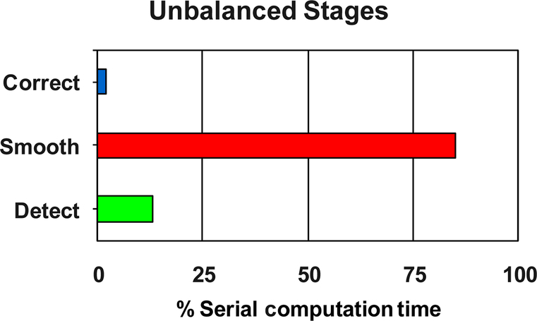
We will start with Step 2: Sequential analysis. Fig. 43 shows that the three processing steps are unbalanced when it comes to total processing load. The “Smooth” function dominates the processing, followed by the “Detect” function and then the “Correct” function. By looking at the code above, we can also come to the conclusion that each function is embarrassingly data parallel. There is constant work per pixel in this algorithm, but also a very different amount of work per function (as can be seen in Fig. 43). This is also the time to make sure that you are only using thread-safe C libraries in this function, as we will be migrating this to multicore software using threads.

Let’s move on to Step 3: Exploration. As mentioned previously this is the step where we explore different parallelization strategies such as:
- • Quick analysis/design, coding, and verification iterations
- • Favor simplicity over performance
- • Verify each iteration
- • Focus on dependencies and decomposition granularity
We decompose to expose parallelism. Keep in mind these rules:
- • Prioritize hotspots
- • Honor dependencies
- • Favor data decomposition
Remember we may also need to “recompose” (we sometimes call this agglomeration) considering:
- • Workload granularity and balance
- • Platform and memory characteristics
During exploration, don’t overthink it. Focus on the largest, least interdependent chunks of work to keep N cores active simultaneously. Use strong analysis and visualization tools to help you (there are several of them we will talk about later).
Let’s move on to Step 4: Optimization and tuning. We will follow these important rules of thumb during the optimization and tuning phase:
- • Follow good software-engineering practices
- • Code incrementally
- • Code in order of impact
- • Preserve scalability
- • Don’t change two things at once
In this step you must also verify changes often. Remember, parallelization introduces new sources of error. Reuse sequential tests for functional verification even though the results may not be exact due to computation order differences. Check for common parallelization errors such as data races and deadlock. Perform stress-testing where you change both the data as well as the scheduling at the same time. Perform performance bottleneck evaluation.
8.2 Data Parallel; First Attempt
The strategy for attempt 1 is to partition the application into N threads one per core. Each thread handles width/N columns. The different image regions are interleaved. We create a thread for each slice as shown in line 10 of the code below and then we join them back together in line 13. How this is partitioned is shown in Fig. 44.

1 void *edge_detect(char unsigned *out_pixels, char unsigned *in_pixels,
2 int nrows, int ncols) {
3 ed_arg_t arg[NUM_THREADS];
4 pthread_t thread[NUM_THREADS];
5 int status, nslices, col0, i;
6 nslices = NUM_THREADS;
7 for (i = 0; i < nslices; ++i) {
8 col0 = i;
9 pack_arg(&arg[i], out_pixels, in_pixels, col0, nslices, nrows, ncols);
10 pthread_create(&thread[i], NULL, edge_detect_thread, &arg[i]);
 11 }
 12 for (i = 0; i < nslices; ++i) {
 13 pthread_join(thread[i], (void *)&status);
14 }
15 return NULL;
16 }
How does this work? Well, not so well. I have introduced a functional error into the code. Diagnosis (Fig. 45) shows that I have introduced a RAW data dependency. Basically there is a race condition in which Smooth0 can read the image data before being written by the Correct function. You can see this error in Fig. 46.


8.3 Data Parallel; Second Attempt
Let’s try this again. The fix to this specific problem is to finish each function before starting the next to prevent the race condition. What we will do is “join” the threads after each function before starting the subsequent function to alleviate this problem. The code below shows this. We create threads for the Correct, Smooth, and Detect functions in lines 3, 8, and 13, respectively. We add “join” instructions at lines 5, 10, and 15. We can see how this works graphically in Fig. 47.

1 for (i = 0; i < nslices; ++i) {
2 pack_arg(&arg[i], out_pixels, in_pixels, i, nslices, nrows, ncols);
3 pthread_create(&thread[i], NULL, correct, &arg[i]);
4 }
5 for (i = 0; i < nslices; ++i) pthread_join(thread[i], (void *)&status);
6 for (i = 0; i < nslices; ++i) {
7 pack_arg(&arg[i], in_pixels, out_pixels, i, nslices, nrows, ncols);
8 pthread_create(&thread[i], NULL, smooth, &arg[i]);
9 }
10 for (i = 0; i < nslices; ++i) pthread_join(thread[i], (void *)&status);
11 for (i = 0; i < nslices; ++i) {
12 pack_arg(&arg[i], out_pixels, in_pixels, i, nslices, nrows, ncols);
13 pthread_create(&thread[i], NULL, detect, &arg[i]);
14 }
15 for (i = 0; i < nslices; ++i) pthread_join(thread[i], (void *)&status);
This is now functionally correct. One thing to note. Interleaving columns probably is not good for data locality, but this was easy to get working. So let’s take the “make it work right, then make it work fast” approach for the moment.
8.4 Task Parallel; Third Attempt
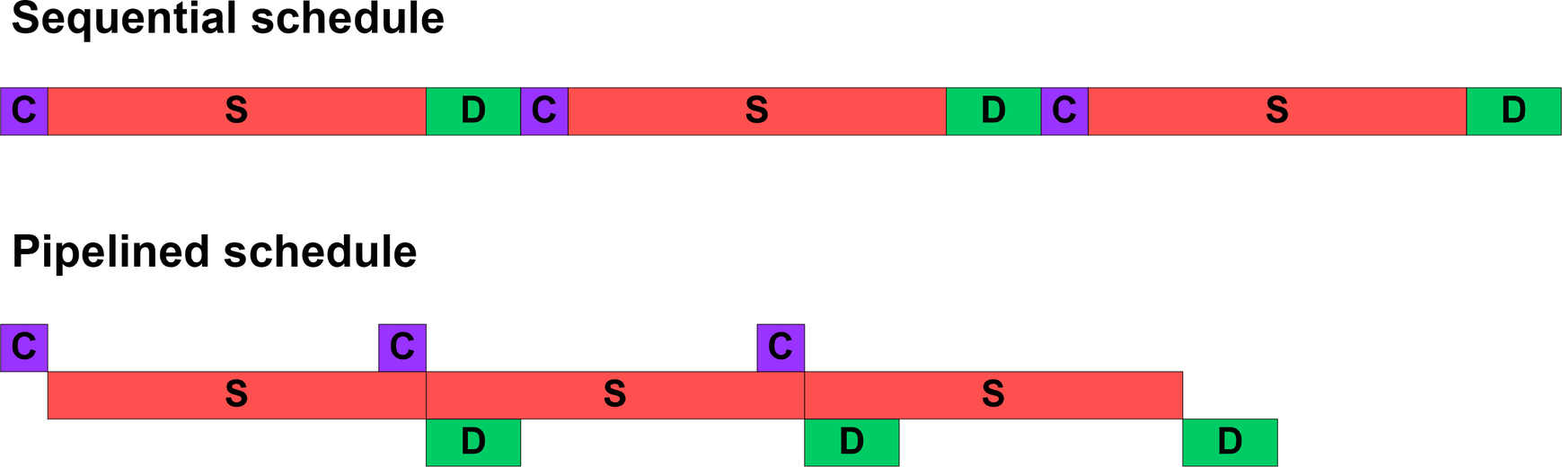
The next strategy is to try to partition functions into a simple task pipeline. We can address the load-balancing concern mentioned earlier by delaying the Smooth and Detect functions until enough pixels are ready. Fig. 48 shows this pipelining approach.

The code for this is shown below. We create our queues in lines 3 and 5. Three threads are created for each function in the algorithm in line 7. We fill our queues in lines 10 and 11, and then join the threads back together in line 13.
1 stage_f stage[3] = { correct, smooth, sobel };
2 queue_t *queue[4];
3 queue[0] = queue_create(capacity);
4 for (i = 0; i < 3; ++i) {
5 queue[i + 1] = queue_create(capacity);
6 pack_arg(&arg[i], queue[i + 1], queue[i], nrows, ncols);
7 pthread_create(&thread[i], NULL, stage[i], &arg[i]);
8 }
9 while (*in_pixels) {
10 queue_add(queue[0], *in_pixels ++);
11 } queue_add(queue[0], NULL);
12 for (i = 0; i < 3; ++i) {
13 pthread_join(thread[i], &status);
14 }
The results are improved throughput but not latency. The throughput is limited by the longest stage (1/85% = 1.12x). This approach would be difficult to scale with a number of cores. The latency is still the same but, like a pipeline, throughput improves. Remember that the stages are very unbalanced, so performance is not very good (Fig. 49). We could consider doing data parallelism within the longest stage to better balance the stages. A comparison of sequential and pipelined schedules is shown in Fig. 50.
8.5 Exploration Results
So far we have some interesting exploration results. We should go with the data decomposition approach. We should match the number of threads to the number of cores, since the threads are compute intensive with few data dependencies to block them. There are still some tuning opportunities that we can take advantage of. We have seen some interleaving concerns in one of our approaches and experienced some delay required for the pipelining design.
8.6 Tuning
We eventually want to identify and optimize performance issues. These could include thread stalls, excessive synchronization, and cache thrashing.
This is where we iterate and experiment. Vary the number of threads and number of cores. Look for ways to minimize locking. Try to separate threads from tasks in different ways to see the impact.
Analysis shows the results of this recent approach made performance worse than the sequential code (Fig. 51)! Diagnosis shows false sharing between caches and significant performance degradation.

8.7 Data Parallel; Fourth Attempt
Let’s try a new strategy. Let’s partition the application into contiguous slices of rows. This should help with data locality and potentially eliminate the false-sharing problem as well. The code for this is shown below. We will refactor the code to process slices of rows for each thread for each function. We create the row slices for the Correct function in lines 1–4, then create the threads in line 5. We do a similar thing for the Smooth and Detect functions before joining them all back together again in line 26.
1 for (i = 0; i < nslices; ++i) {
2 row0 = i * srows;
3 row1 = (row0 + srows < nrows)? row0 + srows : nrows;
4 pack_arg(&arg[i], out_pixels, in_pixels, row0, row1, nrows, ncols);
5 pthread_create(&thread[i], NULL, correct_rows_thread, &arg[i]);
6 }
7 for (i = 0; i < nslices; ++i) {
8 pthread_join(thread[i], (void *)&status);
9 }
10 for (i = 0; i < nslices; ++i) {
11 row0 = i * srows;
12 row1 = (row0 + srows < nrows)? row0 + srows : nrows;
13 pack_arg(&arg[i], in_pixels, out_pixels, row0, row1, nrows, ncols);
14 pthread_create(&thread[i], NULL, smooth_rows_thread, &arg[i]);
15 }
16 for (i = 0; i < nslices; ++i) {
17 pthread_join(thread[i], (void *)&status);
18 }
19 for (i = 0; i < nslices; ++i) {
20 row0 = i * srows;
21 row1 = (row0 + srows < nrows)? row0 + srows : nrows;
22 pack_arg(&arg[i], out_pixels, in_pixels, row0, row1, nrows, ncols);
23 pthread_create(&thread[i], NULL, detect_rows_thread, &arg[i]);
24 }
25 for (i = 0; i < nslices; ++i) {
26 pthread_join(thread[i], (void *)&status);
27 }
8.8 Data Parallel; Fourth Attempt Results
The results of this iteration are better. We have good localization of data and there is good scalability as well. Data locality is important in multicore application. Traditional data layout optimization and loop transformation techniques apply to multicore since they
- • minimize cache misses
- • maximize cache line usage
- • minimize the number of cores that touch a data item
Use the guidelines discussed earlier to achieve the best data locality for the application and significant performance results will be achieved. Use profiling and cache measurement tools to help you.
8.9 Data Parallel; Fifth Attempt
We are now at a point where we can continue to make modifications to the application to improve cache performance. We can split rows into slices matching the L1 cache width of the device (an example of this is blocking where the image can be decomposed into the appropriate block sizes as shown in Fig. 52). We can process rows by slices for better data locality. In the end, additional data layout improvements are possible. Some of these could have been sequential optimizations, so make sure you look for those opportunities first. When migrating to multicore it makes it easier having already incorporated key optimizations into the sequential application.

8.10 Data Parallel; Work Queues
As an additional tuning strategy we can try using work queues (Fig. 53). In this approach we attempt to separate the number of tasks from the number of threads. This enables finer grained tasks without extra thread overhead. Locking and condition variables that can cause extra complexity are hidden in work queue abstractions.

When we use this approach the results get better as slices get smaller (Fig. 54). The key is to tune empirically. In this example we sacrificed some data locality—the work items are interleaved, but empirically this is minor. The results are improved load balancing, some loss of data locality, easy-to-tune thread, and work item granularity.

1 #define SLICES_PER_THREAD 5
2 nslices = NUM_THREADS * SLICES_PER_THREAD;
3 srows = nrows / nslices; if (nrows % nslices) ++srows;
4 crew = work_queue_create("Work Crew", nslices, NUM_THREADS);
5 for (i = 0; i < nslices; ++i) {
6 r0 = i * srows;
7 r1 = (r0 + srows < nrows)? r0 + srows : nrows;
8 pack_arg(&arg[i], out_pixels, in_pixels, r0, r1, nrows, ncols);
9 work_queue_add_item(crew, edge_detect_rows, &arg[i]);
10 } work_queue_empty(&crew);
8.11 Going too Far?
Can we do even more? Probably. We can use task parallel learning to compose three functions into one. We can do some more complex refactoring like lagging row processing to honor dependencies (Fig. 55). This could lead to a threefold reduction in thread creates and joins. This is possible with only minor duplicated computations at the region edge. This modest performance improvement comes with increased coding complexity. See the code below to implement lag processing in this application.

This code is certainly more efficient, but it’s noticeably more complex. Is it necessary? Maybe or maybe not. Is the additional performance worth the complexity? This is a decision that must be made at some point. “Excessive optimization” can be harmful if the performance is not needed. Be careful with “premature optimization” and “excessive optimization.”
1 void *edge_detect_rows(pixel_t out_pixels[], pixel_t in_pixels[],
2 int row0, int row1, int nrows, int ncols) {
3 int rc, rs, rd, rs_edge, rd_edge;
4 int nlines, scols, c0, c1, i;
5 pixel_t *corrected_pixels, *smoothed_pixels;
6 corrected_pixels = MEM_MALLOC(pixel_t, SMOOTH_SIDE * ncols);
7 smoothed_pixels = MEM_MALLOC(pixel_t, DETECT_SIDE * ncols);
8 // determine number of line splits
9 nlines = ncols / CACHE_LINESIZE;
10 scols = ncols / nlines;
11 if (ncols % nlines) ++scols;
12 for (i = 0; i < nlines; ++i) {
13 c0 = i * scols;
14 c1 = (c0 + scols < ncols)? c0 + scols : ncols;
15 log_debug1("row %d:%d col %d:%d
", row0, row1, c0, c1);
16 for (rc = row0; rc < row1 + SMOOTH_EDGE + DETECT_EDGE; ++rc) {
17  if (rc < nrows) {
18  correct_row(corrected_pixels, in_pixels, rc % SMOOTH_SIDE, rc,
20   c0, c1, ncols);
21  }
22  rs = rc - SMOOTH_EDGE;
23  if (0 <= rs && rs < nrows) {
24  rs_edge = (rs < SMOOTH_EDGE || nrows - SMOOTH_EDGE <= rs) ? 1 : 0;
25  smooth_row(smoothed_pixels, corrected_pixels, rs % DETECT_SIDE,
26   rs_edge, rs % SMOOTH_SIDE, SMOOTH_SIDE, c0, c1, ncols);
27  }
28  rd = rs - DETECT_EDGE;
29  if (0 <= rd && rd < nrows) {
30 rd_edge = ((rd < DETECT_EDGE) ? -1 : 0) +
31     ((nrows - DETECT_EDGE <= rd) ? 1 : 0);
32  detect_row(out_pixels, smoothed_pixels, rd, rd_edge,
33   rd % DETECT_SIDE, DETECT_SIDE, c0, c1, ncols);
34 } } }
35 MEM_FREE(corrected_pixels);
36 MEM_FREE(smoothed_pixels);
37 return NULL;
38 }