
Machine Learning at the Edge
Markus Levy NXP Semiconductors, Eindhoven, The Netherlands
Abstract
In this chapter we start by introducing machine learning (ML). We explain the terminology such as supervised and unsupervised ML. We explain the ML tasks called classification and regression. Then we introduce algorithms such as nearest neighbor or support vector machine (SVM), and speak about decision trees and in reference to an example of decision trees we explain ensemble techniques as well as boosting and bagging techniques.
Keywords
Artificial intelligence; Machine learning; Semantic gap; Data augmentation; Neural network; Classification; Regression; CNN; RNN
1 Introduction
In this chapter we start by introducing machine learning (ML). We explain the basic terminology such as supervised and unsupervised ML. We explain the basic ML tasks called classification and regression. Then we introduce basic algorithms such as nearest neighbor or support vector machine (SVM), and speak about decision trees and in reference to an example of decision trees we explain ensemble techniques as well as boosting and bagging techniques.
In the second part of this chapter we focus on neural nets (NNs) and explain the basic concept of a neuron and how neurons are arranged into networks and how the basic mechanics of NNs work. Then we examine the learning process in these networks and the associated backpropagation algorithm.
This is an appropriate place to insert a disclaimer. Machine learning (mainly the domain of deep learning) is changing so rapidly that what you read might not be 100% valid. The best approach to getting the most out of this chapter is to take it as a starting point, learn the principles, follow the suggested literature references, and see if they are cited in fresh papers—the optimum way to keep up to date with current state-of-the-art information.
We assume that a reader has basic knowledge of linear algebra, probability and statistics, calculus, and optimization.
1.1 Coding Examples
In this chapter you will find code examples. However, unlike the other chapters in this book these examples will be written in Python, primarily because most of the ML libraries and supporting tools are based on this programming language. We are aware that Python is slower than C ++ and similar languages. On the other hand, most of the libraries, like NumPy [1], are written in C ++ and well optimized and Python is just an interface enabling much easier and faster development, and the computational overhead is negligible. Python code is also more readable and shorter allowing us to provide more examples. Furthermore, Python is more suitable for ML when there is a need for a fast way to test hypotheses. Once a proper way is found Python be rewritten and optimized into C ++ format.
To be able to run the code examples the reader needs to have access to Python 3.7.* and the following libraries: NumPy, Matplotlib, Scikit-Learn, PyTorch, torchvision. These are widely used on most platforms, and installation issues can be solved with solutions found using Google Search.
1.2 The Machine Learning Revolution
Lately the primary focus on machine learning has been on neural networks (NNs) and so-called deep learning. The main reasons for this focus are:
- ⦁ There are huge data sets available and the information continues to expand.
- ⦁ Processing hardware is more powerful than ever before.
- ⦁ Industry experts have discovered that deep NNs are able to outperform the current state-of-the-art techniques that have been handcrafted and tuned for decades. Previously, no one was able to sufficiently train these deep architectures because there just weren’t enough data or processing power to do it.
In this chapter we will discuss deep learning and the methods used before its widespread adoption. These classical methods are usually lightweight in size and might also be faster than NNs. For some applications they might provide comparable accuracy, but with much smaller costs and it would be a huge mistake to ignore them. Sometimes they are also used in combination with neural nets.
2 What Is Artificial Intelligence
Artificial intelligence (AI) has many possible definitions. One is that it is an ability of a computer or computer-controlled device to perform tasks commonly associated with intelligent beings. Herein lies the first problem—it is not easy to define an intelligent being—but it should probably include an ability to reason, discover meaning, generalize, and learn from experience.
There is a famous Allan Turing test [2] in which artificial intelligence is accepted when a human observer is not able to distinguish the results of a given program from results provided by a human performer. Today there are chatbots able to converse on various topics that might be indistinguishable from a human. In some specific domains machines have even surpassed human performance, but only on a well-trained, given task (e.g., image classification, translation). If we want to speak about general AI (i.e., a program able to perform any task a human can do), we are still far away from achieving such capabilities. Current complex solutions are usually an assembly of various subsystems.
AI is an interesting domain because it represents a combination of mathematics, computer science, engineering, neuroscience, philosophy, and other studies—thereby making it difficult or impossible for any one person to be a complete AI expert. As you’ll see later in this chapter the good news is that there are a growing number of open-source technologies and tools that are helping to bring AI to the masses.
3 What Is Machine Learning?
Machine learning, a field of computer science and a subset of artificial intelligence (AI), is comprised of many algorithms. These algorithms have in common an ability to learn (or be trained) to perform a given task based on the data provided. It can be viewed as a prediction tool that can deal with visual, textual, vibrational, and many other types of input data. For example, given an image of a face ML can predict whether the image is that of a man or woman. Given newsfeeds that include a previous price and current price of gold ML can predict the gold price in the next hour. Given sensory data, like vibrations, ML can detect or predict a motor failure.
This raises another important aspect to consider since predictions are guesses. Algorithms will never be 100% correct and it is difficult to predict when they will fail (however, the better the training, the better chance the prediction is closer to 100%). Predictions can easily fail when presented with kinds of data the algorithm has never previously “seen,” especially if the training was not generalized properly. The main issue is that most of the algorithms are not aware of “not being sure” (e.g., when we train a system to label images either “pigs” or “cows” and we don't introduce a category like “others,” it cannot do better than label an image of car with the high probability of being a “pig” or a “cow” (in the best case it will be irresolute—giving 50% to both).
In machine learning no code is written except for the implementation of training and the inference of an algorithm. There are no handcrafted rules. If you consider face detection, for example, we as humans don’t really know how to do it, it just happens somewhat automatically. It would be difficult (if not impossible) to provide instructions showing a person how go about face recognition. If a person had the ability to learn we would try to teach them by sharing images, and on the images they would point to positions where they think the face is present. Then we would provide them with an answer (e.g., in this image there is no face or the face is more to the right). ML is also called pattern recognition since that is what you are seeking—patterns.
In this chapter we won't discuss a concept called general artificial intelligence. Algorithms described in this chapter can perform one exact task—even if the machine-learning algorithms are an assembly of many components to perform complex tasks, like driving, you won't expect the same machine to be able to clean your table and put dishes into your dishwasher.
This approach is called supervised learning, which represents most ML algorithms. When we want to categorize ML one criterion is based on how much we know about provided data:
- ⦁ Supervised—Learning with a teacher. In supervised learning in addition to providing data (e.g., images) we also obtain the desired results (e.g., x, y, width, height—parameters of a rectangle defining the position of a face in the image). These results are usually called ground truth. Such images are called labeled and/or annotated.
- ⦁ Unsupervised—Learning without a teacher. In this case we are given unlabeled data only. Based on assumptions there are different approaches to choose such as clustering, anomaly detection, autoencoders, etc.
- ⦁ Semisupervised—As the name suggests, this lies between supervised and unsupervised. Typically, we get a small set of labeled data and a large unlabeled data set usually because of the high cost of acquiring labeled data. Semisupervised learning attempts to use this combined information + assumptions (e.g., continuity—the probability of having the same label is higher for data points closer to each other). It also outperforms unsupervised algorithms in situations when labels are completely removed and outperforms supervised algorithms running only on a small subset of data.
Intuitively, we can think of the semisupervised learning problem as an exam and labeled data as the few example problems that the teacher solved in class. The teacher also provides a set of unsolved problems. In this setting these unsolved problems are a take-home exam and you want to do particularly well on them. In the inductive setting these are practical problems of the sort you will encounter in the in-class exam. The supervised analogy would be almost the same, but without the unsolved, take-home examples.
The following sections refer to a supervised machine that can be summarized as: given data X and corresponding results Y find model parameters θ such that they will minimize the given loss function L (loss function explained later, but it basically measures the difference between prediction and ground truth). Herein the two most common tasks are classification and regression.
In classification, for a given data X, predict the correct label/category Y. The classification task is further divided into concrete categories:
- ⦁ In binary classification inputs are classified into two groups (classes). Binary classification is considered a better understood problem, while multiclass classification is more complex. Some algorithms are built based on this relaxed property (only two classes) and are not able to solve tasks with three or more classes. As an example of binary classification—based on weight and height predict whether we observe a basketball player or a jockey. Another example might be given some email messages and their headers—decide if it is or is not SPAM.
- ⦁ Multiclass classification makes binary classification more general, and the number of classes is bigger. For example, given a face image classify which friend it is (e.g., John, Bruno, Markus, Philip, or Rob). It is not rare for binary classification algorithms to be used in multiclass classification tasks in “one vs. all” (OvA) or “one vs. one” (OvO) mode [3]. OvA is when a single binary classifier is trained per class with the samples of that class being positive samples and all the others being negative. OvO is when a single binary classifier is trained for all class pairs, then during the prediction phase all classifiers predict and the result is based on “voting.” This allows using binary classifiers, like SVM, in multiclass tasks as well.
- ⦁ Multilabel classification assigns to each data sample a set of labels. For example, given categories (classes) {blues, rock, funk, jazz, hip-hop, classical, country, R&B, soul} and given the audio file return all genres that it can be categorized into. A valid result might be {blues, rock, soul}, for example (Fig. 1).

Fig. 1 The difference between regression and classification task. Regression is when we detect face position in an image or predict age. Binary classification is when deciding if a given face image is a man or woman. Multiclass classification would be when we want to decide whether the face is happy, neutral, or sad.
For regression tasks the goal is to predict one or multiple continuous values. For example, if the algorithm is detecting a face in an image we want to predict values (x1, y1), (x2, y2), the corner points of a bounding box defining the face’s position. Algorithms used for regression are usually different than those used for classification tasks, but some can be used for both (e.g., decision trees, neural nets).
One interesting thing to note when talking about classification tasks is object/region detection vs. classification. In many cases a key step is finding the region(s) (which might be a regression) of an image (camera or stored picture) where something exists that is worth classifying. This is because an HD image (say 1920 × 1080 or bigger) is a lot of pixels—doing a detection to locate possible things of interest is an important consideration (especially as you can downsample to do this). Likewise, this comes up in voice recognition (waiting for voice band and sound that is not continuous or background), control systems (waiting for plant to change), sensing classifications (e.g., metal fatigue, etc.). Detection as a form of reduction to a small set is really important for embedded systems as it makes the problems practical as well as saving power (in many cases).
One popular way of carrying out a vision task is via background/foreground segmentation where in the simplest case a background model is computed as an average of previous frames, and the current frame is pixel-wise compared with this model. When the difference is bigger than some threshold a pixel is considered to be a foreground. This is not an ML approach as it is an exact algorithm.
3.1 Bias vs. Variance Trade-off
There are two sources of error that prevent supervised learning algorithms from generalizing beyond their training set:
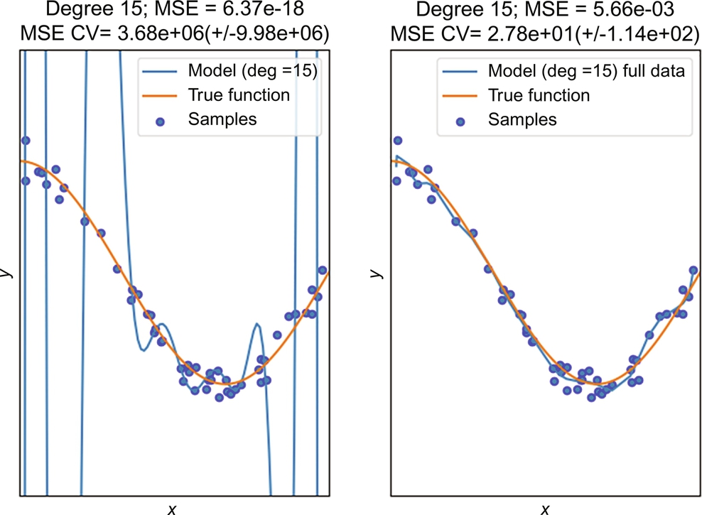
- ⦁ Bias is an erroneous assumption in the learning algorithm. It can cause relevant relations between features (input data) and outputs (e.g., fitting polynomials of degree 1 (linear) into data with quadratic relations) to be missed. This issue is also called an underfitting problem.
- ⦁ Variance is an error that results from sensitivity to small fluctuations in the training set. It can cause an algorithm to model random noise in the training data and somehow mimic memorizing the dataset. It is also called an overfitting problem.
Bias can be prevented by using a more complex model, but as the number of parameters increases the model will be more prone to overfitting. Overfitting can be prevented with more data. There is always some trade-off between bias and variance when we are choosing the proper model. To support intuition see Figs. 2 and 3.

Regularization techniques are another way to prevent overfitting. These techniques add an associated cost into the loss function for each parameter used. This allows the model to have the flexibility to choose the proper complexity. There is no silver bullet for choosing a proper technique, and it usually requires lots of experience and intuition to set up everything properly.
To support the intuition behind overfitting go back to the example of learning to detect faces in images—what happens if we only show 10 examples to a lazy student with a good memory (big number of model parameters). The student will probably find it easier to memorize the answer instead of learning to generalize/use reasoning. Then we can determine whether the student was able to generalize if we show him previously unseen examples. If he just memorized the question and answers, then he will fail. The same approach is used in machine learning, whereby the previously unseen data are called test data, and with this approach we can estimate how the algorithm will perform in the future (additional details are provided in the next section).
4 Feeding Your Brain—Data
In machine learning data are crucial and can have various forms including audio/sound, images, videos, aggregated data/statistics, and text strings. What is important is that in the end the data should be preprocessed and combed into a numerical matrix X where each row represents a single data sample. The annotations should be preprocessed into a vector/matrix y where each row bears the required result(s) for the data sample in the matrix X.
4.1 Data Are Crucial
- ⦁ If you don’t have enough data, then state-of-the-art algorithms won’t help you.
- ⦁ If you don’t have enough data, then complex models (with a high number of parameters) will tend to overfit (see Section 3.1) and fail dramatically when deployed.
The natural question arises: How many data are enough? The higher the model’s complexity, the higher the demand for data. There are some theoretical boundaries, like the Vapnik-Chervonenkis theory for VC dimension [4], providing rough estimates. Some basic rules are that we need at least k independent examples for each class; there must be more independent examples than the number of input features and more independent examples for each parameter in the model. If we take, for example, an input to be an image of size 500 × 500 × 3, we at least know that we should have more than 0.75 M images to train a given model. Another approach to estimate the required amount of data is to look at similar problems and published papers.
Another thing we should be aware of is that a lot of ML algorithms assume that data are independent and identically distributed (i.i.d.). This is a terminology from probability theory and statistics. I.i.d. means that each random variable has the same probability distribution as the others and all are mutually independent. But what happens when we violate that? What happens when we have fewer training data? Usually, the model still learns something, but might be more prone to overfitting. This is task dependent as well as algorithm dependent.
4.2 Data Preprocessing, Grooming, and Preparation
The goal of data preprocessing is to prepare data into a “tabular” numerical arrangement. This means that ultimately all data must be transformed into numbers. For example, this might mean encoding categorical variables using one-hot encoding. Tabular means that each data sample is in a row, whereas columns represent features and a few of the last columns have the right answers (e.g., class number).
The entire process can be reduced to:
- ⦁ Data cleaning—a process in which wrongly completed questionnaires, invalid experimental data, or data not passing through logical control are removed.
- ⦁ Data labeling and tagging—for cases where some of the data are unlabeled we must “get our hands dirty” and create annotations. This step is usually also educative because we can learn a lot about the nature of the given task. This task is usually outsourced.
- ⦁ Augmentation—allows us to automatically enlarge our data set (explained later in more detail).
- ⦁ Selection of training, validation, and testing sets (described later).
- ⦁ Normalization—this step normalizes data. The reason is that most algorithms work better after this step. The only algorithm class (of those covered in this chapter) that doesn’t need this step are decision trees (see end of Section 6 for an explanation of why the algorithm might fail without normalization).
- ⦁ Feature extraction (covered later).
4.3 Training/Test and Validation Data Split
To prevent overfitting, data are usually divided into three categories. The first and biggest category is the training data set; it is usually 80%–90% of the size of the regular data set. To have a balanced data set the training data set is typically pseudorandomly chosen from the whole data set. For example, 80% are randomly chosen from each class to ensure all classes are represented.
The remaining 10%–20% of the data are typically divided into two equal-sized data sets—a test set and a validation set. The test set will only be used in the final process to evaluate and predict how well the model generalizes for new data (i.e., not used during the training phase!). The validation set is used to tune hyperparameters for a given ML algorithm.
A slightly more complex but commonly used technique is called k-fold cross-validation [5]. This technique divides the data set into k balanced folds (whereby the user determines the number of folds k and balanced means in which the percentage distribution of classes stays approximately the same proportion as in the full data set). Then the training process is done for all except the kth fold (this is used as the test and validation set). The entire process is done k times. By measuring the accuracy average and standard deviation we get a much better estimate on how the model generalizes. Commonly used values of k are between 5 and 10. Typically, higher values are better, but this increases the training time. This k-fold technique is not commonly used with neural networks because the training time is usually more demanding than a suitable non-NN algorithm.
4.4 Semantic Gap
Humans have a very advanced perception of the world around us. For example, when we see something we don’t think about each photon or atom. Instead, we perceive objects, faces, textures, etc. The same applies to audio; we don’t think about frequencies in time, instead we perceive words from which we build sentences and on top of that we reason.
On the other hand, observe how a machine sees the world (Fig. 4). The bottom section of the images are 10 × 10 matrices representing the highlighted red blocks. Notice how different the matrices look even after rotating the block by only 2°, although humans have no problem recognizing the rotated image. This demonstrates the huge semantic gap within data and how humans interpret them. For obvious reasons we want to design our systems to be resilient to such changes (e.g., slight rotations, translations, noises, intensity changes) (Fig. 5).

4.5 Data Augmentation
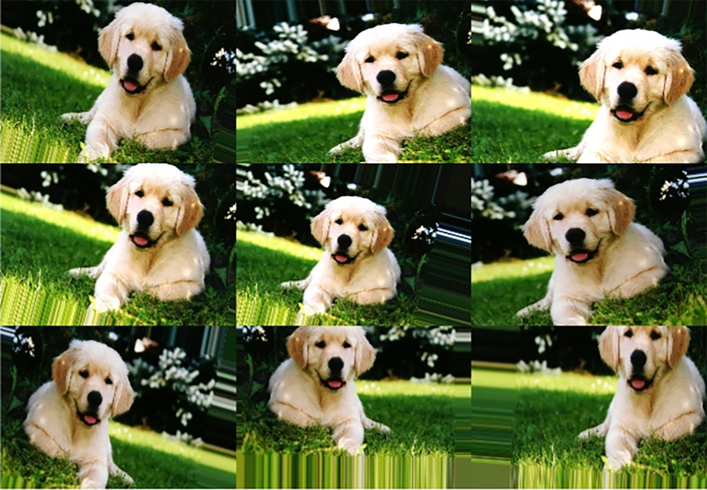
We’ve learned that data are crucial and that usually it is difficult to obtain enough training data to achieve close to 100% accuracy on predictions. Data augmentation is a great way to increase the number of training examples. Using an example of image classification we want to classify an image of a dog as a dog even if the image is horizontally flipped, contains a little random noise, or is scaled, translated, or rotated. In computer vision these data modifications are straightforward and applicable beyond traditional image classification (e.g., it can be used for regression like object detection). The only rule is that the augmented image still maintains the same label or at least we know how to change the label (e.g., in the case of object detection, if we rotate an image slightly, we must change the object’s digital position as well). It is possible to do the same for audio (e.g., adding background noise, increasing the tempo, phase shifting, etc.). Similar techniques can be applied to other domains.
Why does data augmentation work? Looking at Fig. 4 we don’t think the image changed significantly, but from the computer’s perspective the data matrix is completely different even when small changes are applied. This process is artificially accomplished by adding more examples of the same class, and more examples should help to prevent overfitting. Furthermore, compared with manual labeling the computational cost of augmentation is negligible.
4.6 Introducing an Image Classification Problem
The best way to learn something is to apply what you’ve already learned to solve a problem. In this section we will apply ML algorithms to an image classification task (we’ll train our own convolutional neural net or CNN). We will use a task from the computer vision domain because it is more intuitive to visualize what is happening (Fig. 6).
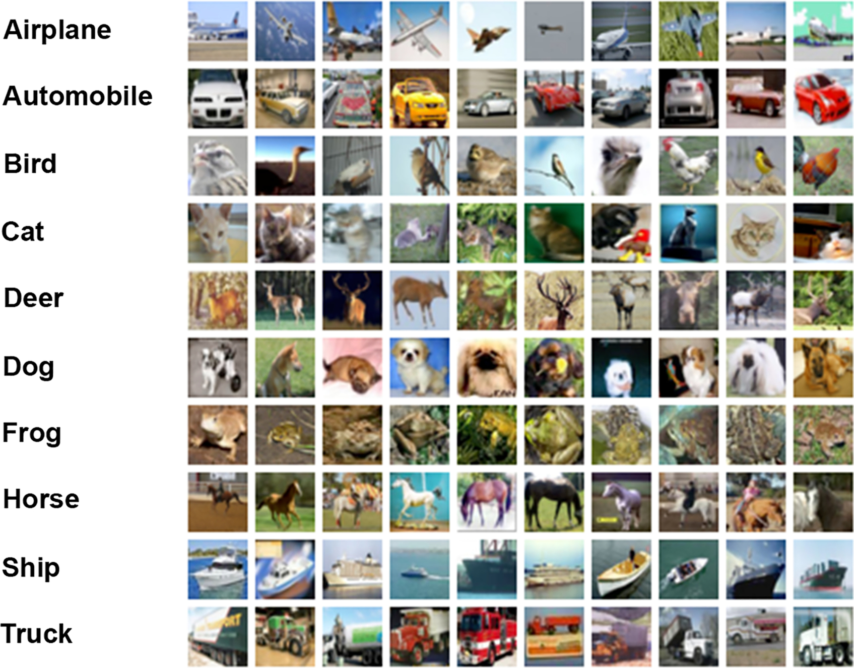
The CIFAR-10 data set is a relatively small, publicly available data set with 32 × 32 color images sorted into 10 different classes (e.g., airplane, automobile, dog). CIFAR-10 is considered a sandbox data set that is useful for testing but not real-world inferencing, replacing the previously popular MNIST example (28 × 28 images of handwritten digits). The simple MNIST model has become well understood (many recent algorithms have less than 0.25% accuracy error whereas state-of-the-art algorithms on CIFAR-10 achieve rates of around 2%).
4.7 Feature Extraction
For any type of machine learning the input data should be preprocessed. Take audio classification, for example—the incoming audio signal must be filtered to remove ambient noise. For vision applications various types of filtering or color conversion might be utilized to enhance specific colors or lines.
Here we list a few commonly used feature extraction techniques (we can also view feature extraction as a dimensionality reduction): in computer vision a search for key points (e.g., corners, dark/light blobs, etc.) is done and then each key point is described using algorithms like SIFT, SURF, ORB, Tf-idf for text analysis, or MFCCs and MPEG-7 for audio, etc. Handcrafted features can also be utilized.
For image classification, for example, an entire 32 × 32 × 3 image can be unraveled into a 3072 × 1 vector. This vector might be our feature space, the dimensions where the variables live. However, most ML algorithms will suffer from such a big feature space, and this is often referred to as “the curse of dimensionality”—a situation in which data are organized in high-dimensional spaces. The main problem is that as the number of dimensions increases the data points become sparse, statistical significance drops, and this in turn damages the methods that rely on it. A big feature space will also harm the speed of inference as well as training. Finally, another problem of a big feature space in the case of an image is that there is information hidden in the pixel distribution (spatial relations are very important and if you do random permutation of pixels you will no longer be able to recognize the image). If we compare images at the pixel level, there is a huge semantic gap; shifting an image a small amount causes completely different values of the given pixels (refer to Section 4.4). This highlights the fact that we need a better way to represent each image.
An easy and straightforward way to represent images is to make us of a color histogram. A histogram divides a given range into bins and then counts the number of occurrences in each bin. For example, we can divide each color channel into k bins and compute how many pixels of a given intensity in that given channel are present in an image. Using this approach we can reduce the feature space from 3072 × 1 into a much more manageable 3k × 1 vector. See examples of histograms in Fig. 7.

4.8 A Baseline
In the following sections we will introduce several famous ML algorithms, but before starting let’s think about a small experiment. What about having a naive classification algorithm returning a class randomly? This algorithm will have an accuracy of 1/K, where K stands for the number of classes. It is good to consider this as a baseline and sanity check. When our algorithms perform below this number it is an indication of something being broken. Therefore, it is good practice to have these types of sanity checks included during development.
5 Support Vector Machine
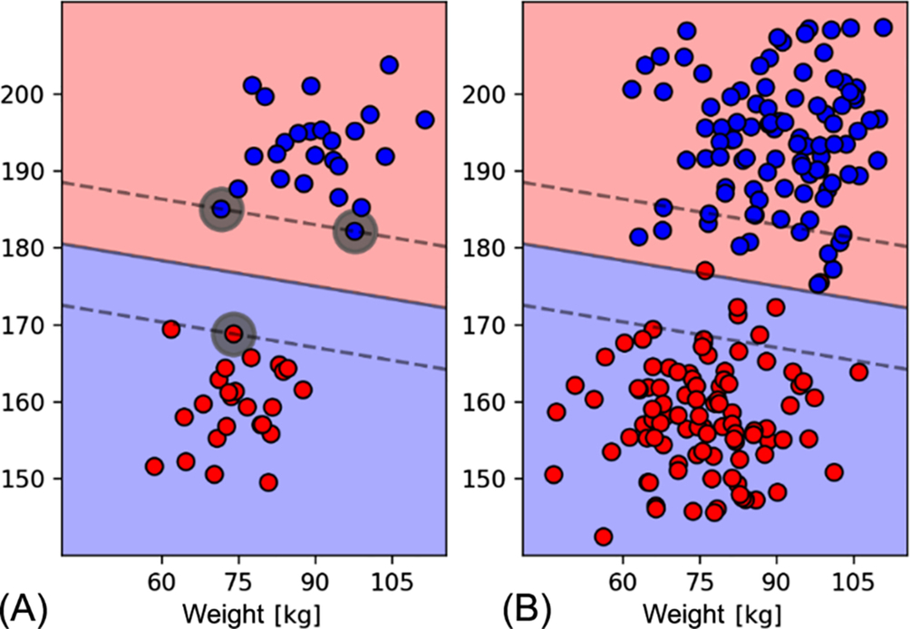
Here’s a task—given weight and height, classify whether an observed man is a jockey or basketball player. We are also provided with training examples (see Fig. 8A). Let’s consider red to be jockeys and blue to be basketball players. A simple way to solve this task algorithmically would be to define a line and everything to the left is considered class 1.

Mathematically, for the linearly separable case any point x lying on the separating line satisfies xTw + b = 0, where w is the vector normal to the line, and b is a shifting constant from the origin. The distance of the line from the origin is ![]() . If we change equality to inequality we have a decision maker: xTw + b ≥ 0 is a jockey and < 0 is a basketball player. If we look at Fig. 8B there is an infinite number of possible lines. Fig. 8B shows that there is an infinite number of possible lines. From Fig. 8C we can see that when we use these three classifiers on real data (not seen during training) some lines are better than the others.
. If we change equality to inequality we have a decision maker: xTw + b ≥ 0 is a jockey and < 0 is a basketball player. If we look at Fig. 8B there is an infinite number of possible lines. Fig. 8B shows that there is an infinite number of possible lines. From Fig. 8C we can see that when we use these three classifiers on real data (not seen during training) some lines are better than the others.
The support vector machine (SVM) algorithm is built on the following idea—choose a line that has the biggest distance to all data points, because such a line will better generalize on the inference. We can enforce this policy by slightly modifying our equation: xTw + b ≥ m, where m is a margin we want to have for all data. If we define our training labels yi as 1 for jockeys and − 1 for basketball players, we can then define the training criteria as yi(xTw + b)≥ m. Using the formulation of distance from the origin of three lines we can show the margin ![]() . Without any loss of generality we can set m = 1, since it only sets the scale of w and b. Now it is clear that if fraction
. Without any loss of generality we can set m = 1, since it only sets the scale of w and b. Now it is clear that if fraction ![]() is maximized the margin M is also maximized (Fig. 9).
is maximized the margin M is also maximized (Fig. 9).
Finding the parameters for the best dividing line can be done by solving for the following quadratic programming problem:
As this is not a convex function t is reformulated in practice as a dual ![]() … , which is convex and hence easier to optimize. Luckily, as an ML engineer you can usually stand on the shoulders of giants and use ML libraries. Usually, we just construct an SVM classifier with given parameters, train it with data, and then use it for class prediction.
… , which is convex and hence easier to optimize. Luckily, as an ML engineer you can usually stand on the shoulders of giants and use ML libraries. Usually, we just construct an SVM classifier with given parameters, train it with data, and then use it for class prediction.
Given this problem definition there is still one issue to resolve. In a case when even one point is positioned in such a way that linear separation is not possible the entire optimization problem won’t work because it won’t be possible to satisfy all the constraints. This is solved by adding a penalty for each data point not satisfying the equation. All these penalties are weighted by parameter C which controls the trade-off between a smooth decision boundary and classifying the training points correctly. It is a hyperparameter of SVM and it is a good idea to try multiple choices. A reasonable starting value is 1.0:

This code sample describes how to train our own SVM classifier. The same code template might be used for any other classifier. The interface is usually the same—construct, fit data, predict.
All these approaches can be easily scaled into higher dimensions, where the line becomes a plane in 3D and a hyperplane in higher dimensions; the math stays the same.
So now we have at least a rough idea how to solve a linearly separable task. But what about a linearly nonseparable task? To see how our approach performs on such a task look at Fig. 10. Linear SVM cannot solve this task, but one way to deal with this issue is to transform the feature space into another format (see example in Fig. 11). We can change the previous code example to use the kernel just by modifying the previous code example around line 15 in the following way:


Further information with detailed proofs of the SVM algorithm can be found in any ML textbook (e.g., [7]), and more information on kernel methods can be found in [8].
6 k-NN (Nearest Neighbor) Algorithm
Nearest neighbor is a very simple, intuitive, and valuable approach to data classification and has been used for many years. Given a query Q and a metric function d(Q, Xi), the nearest neighbor algorithm measures the distance to all training examples (data points) and returns the classification of the closest data point. The algorithm described above is called nearest neighbor—1-NN. An easy modification is to take the closest k and choose the class with the highest number of votes; using this approach class probabilities might be estimated by dividing the number of votes for each class by the number k. The nature of the algorithm means it is capable of solving linearly nonseparable tasks where previously shown SVM methods failed (Fig. 12).

Euclidean distance (also called L2 norm) is a frequently used metric function ( ). However, you can also define your own metric function suitable for the given task—there are no limits.
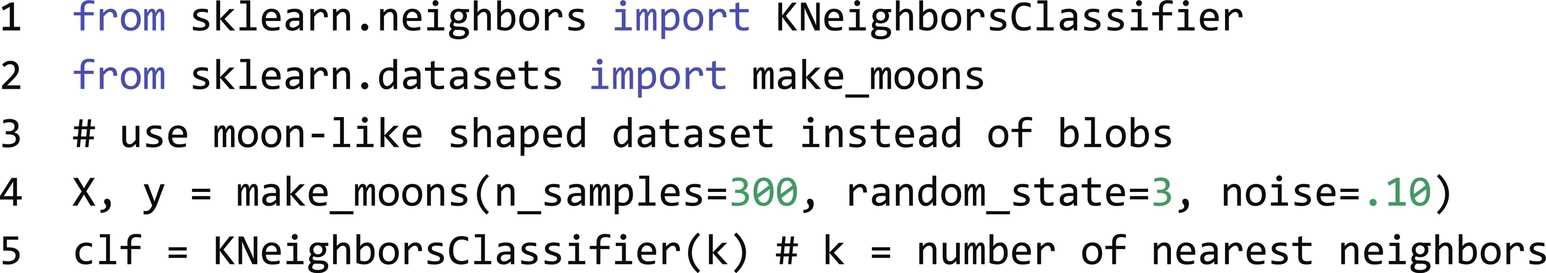
We can use NN Classifier on the previous task from SVM just by changing two lines. The code for generating similar visualizations is inspired by scikit-learn tutorials [9]:
The main advantages of the k-NN algorithm are that it’s an easy implementation, it works on nonlinear cases, and has constant training time O(1) (this stands for big O notation, an upper bound complexity estimation that in this case is constant—not dependent on input size as no actual training is performed). The main disadvantage is that when the number of dimensions increase a lot of data are needed because in high dimensionalities data entries become rare and sparse. Next all training data must be stored and the inference time is O(N), where N is a number of training examples (which means it is slow). These limitations can be overcome by using more advanced data structures like k-dTrees [10], where inference time is on average O(log N) with the worst time is still O(N).
Even though the nearest neighbor method is very simple it can still find use cases where the data dimensionality is low and space is well covered. New attempts have been made to improve this concept (e.g., [11]).
It is important to note that, as described in Section 4.2, most ML benefits derive from data normalization. Let’s return to our example from the SVM section (jockey/basketball player classification). What happens when we have weight measured in kilograms but height in millimeters? The Euclidean distance will change by the same amount whether we add 10 kg or 10 mm, thus information about weight will be mostly ignored.
7 Decision Trees
A decision tree, another important and frequently used concept in ML, is a mathematical structure from graph theory (specifically, it is a directed acyclic graph or DAG). Each tree starts with a root node that branches into descendant nodes. When a node has no descendants it is called a leaf. Binary trees are very common, so-called because each node has up to two descendants. A decision tree implies that a decision function resides in each node, and based on the output flow continues to branch into descendant nodes until a leaf is reached. Decision trees are most commonly used for classification tasks, implying that each leaf holds a class label (or class label distribution) (Fig. 13).

A benefit of decision trees is that once trained the testing phase of a decision tree is relatively fast (O(log N)). Additionally, decision trees can work on nonlinear tasks. Another great value of a decision tree is in the way it can interpret a model (a path to the leaf can be followed and each decision can be interpreted). Interpretability is an important aspect of an algorithm. For example, imagine a task where ML is used to help a doctor with disease diagnosis. There is minimal value in saying: “I think it is cancer”; it’s better if an algorithm can infer there’s cancer with a probability of 98%, allowing a decision to be made based on these criteria.
One disadvantage of decision trees is that they can badly overfit, thus they might not generalize very well (ensemble learning, introduced in the next section, can be applied to overcome this issue).
7.1 Ensemble Learning
We will explain ensemble learning here as it relates to decision trees, but these approaches are general and can/should be used with other algorithms. Ensemble learning usually comes with higher computational and memory cost, but it leads to higher accuracy. In accuracy-critical applications these techniques are also used for computationally intense algorithms like NNs. Ensemble learning is a technique that can make decisions based on multiple models which can be homogeneous (e.g., 10 decision trees) or heterogeneous (e.g., decision tree + SVM + neural network). A heterogeneous example is based on the idea of combining the results of different algorithms, assuming that each has its own strengths and weaknesses. Why does it make sense to use it on homogeneous models? Aren’t the models the same? First, since we can use different hyperparameters for each model they might be slightly different. There is also a technique in which the hyperparameters are the same, and yet it still makes sense (one of them is called a random forest classifier/regressor; see Section 7.3).
7.2 Bagging
Using a technique called bagging (bootstrap aggregating) we combat overfitting by taking k-same models. With this technique we randomly sample a subset of data (e.g., 85%) from the training data set for each model. Then we train the model, perform k predictions, and in the case of a classification task take the argmax. We can also recast this information as a probability distribution over classes. This approach works because each trained model saw just a portion of the data set, thus it cannot fully overfit. In combination with other models it generalizes better on a given task.
7.3 Random Forest
The decision trees concept has many versions, and one of the most frequently used is the random forest approach [12]. This uses the ensemble-learning concept called bagging, but this is not the only randomization performed. During training a vanilla decision tree uses all features to choose which one best divides the data. The random forest approach randomly samples a subset of features in each node (a frequently used subset size is ![]() ,where F is the number of features). This helps prevent overfitting and speeds up the training process. In the end the final decision is based on voting (as in any other ensemble method):
,where F is the number of features). This helps prevent overfitting and speeds up the training process. In the end the final decision is based on voting (as in any other ensemble method):

As mentioned in Section 6 it is easy to reuse the code for classification and use a different algorithm. We can try to do the classification using a random forest with 10 trees. Classifier has many more parameters like max depth. A great way to build intuition about this is to play around with parameters and observe what Classifier does (Fig. 14).

7.4 Boosting
Boosting is another ML technique that produces a prediction model as an ensemble of so-called weaker models. Boosting is done in an incremental way where each new model emphasizes the training data misclassified by the previous model. Sometimes boosting might have better accuracy than bagging, but it might be more prone to overfitting. AdaBoost [13] is an example of a boosting algorithm. Because of its efficiency and flexibility XGBoost [14] is a commonly used implementation of gradient boosting. It is usually good practice to compare multiple approaches (e.g., gradient boosting vs. random forests) on a given problem and choose the better one (using trial and error).
8 Neural Nets
Neural networks are another category of algorithms that are getting lots of attention, but remember you should avoid using them unless your application requires complex classifications (etc.). Classical machine-learning algorithms are easier to train and typically require fewer computations. Anyway, NNs are brain-inspired algorithms known since the 1950s (Warren McCulloch and Walter Pitts created a computational model for NNs based on threshold logic), and the general methodology has not changed significantly over the decades. However, what has changed is the usage model—NNs were previously only useful for PhD mathematicians—now, through a variety of proprietary or open-source frameworks and tools, NNs are in the hands of the masses.
8.1 Motivation
A distinct historical landmark is the 2012 success of AlexNet [6] in the ILSVRC image classification challenge utilizing the ImageNet data set [15]. The task was to classify ImageNet’s images into one of 1000 classes including animals, dog breeds, cello, cradle, car wheel, volcano, seashore. These algorithms were compared using top-5 metrics, which means the top-5 predictions are returned and if the correct class is among them it is accepted as a correct prediction. As seen in Fig. 15 the last successful classic computer vision approach was done in 2011 where there was a 26% top-5 error. The following year AlexNet [6] reduced this error by almost 10%; this ignited the spread and domination of convolutional neural nets (CNNs). In 2014 AlexNet was followed by the larger VGG network [16] as well as the more complex GoogLeNet [17]. Finally, in 2015 the even deeper CNN architecture ResNet [18] outperformed human performance in the top-5 classification tasks (Figs. 16 and 17).


8.2 What Is a Neural Network?
A neural network is a brain-inspired algorithm in which the basic building block is called a neuron—so-called because it is a simplified, mathematical model of a biological neuron. Each neuron has one or more inputs and a single output. Similarly, inputs are called synapses and there are typically other synapses connected to the output—sending information to other neurons. Each synapse is represented by three properties: a starting neuron, a weight, and an ending neuron. The synapse weights are the primary NN parameters. Where does the “magic” occur? Each neuron takes a signal from each input, multiplies it by a synapse weight, and sums these products together (i.e., a multiply-accumulate function).
On top of that, an activation function is applied. The main purpose of an activation function is to bring nonlinearity into the whole system. This is a very important aspect. Compared with a vanilla SVM (which is linear), NN can solve nonlinear tasks. Recall from Fig. 11 that when we want to separate data points it is not possible to do it with a line (this is called linear nonseparability). Thanks to the nonlinearity added in an activation function the NN is projecting (warping/upscaling) its input feature space into a new one where linear separation might be possible in the end.
Another goal of an activation function might be to scale the output into a given range (e.g., < 0, 1 > for a sigmoid function). For more examples of activation functions see Fig. 18. The output of the activation function is then sent to all other connected neurons, multiplied by the respective weights, and so on through each layer of the network.

In general, neurons are connected and form a graph structure called a directed acyclic graph (DAG). DAGs can have almost any imaginable topology. When referring to currently used deep-learning architectures, DAGs are best organized into layers (Fig. 19). Layers are groups of neurons. As we’ll see in the following sections, layers can be more complex than a straightforward fully connected one (which means that each neuron has a connection with all neurons from previous layers). One example of a more complex layer is a convolution layer, which is described in the Section 8.4. The convolution layer is one of the most important concepts in NNs for vision and other tasks.

8.3 How Training Works
8.3.1 Backpropagation—Key Algorithm for Learning
Section 4.3 describes how a training data set can be divided into three subsets. In the first stage of training we’ll start with an untrained NN architecture initialized with pseudorandom weights (actually this random distribution is chosen in a clever way). Training data are then fed into the NN and a feedforward step is applied. From the output we get results that we can use to compute the loss that must be minimized to trend toward the desired result. The question is how to minimize the loss function in an efficient way—this is where backpropagation comes into play (Fig. 20).

Backpropagation is a process in which each parameter/weight of a network is systematically updated to minimize the loss function. An example of a loss function might be a mean squared error (MSE) defined as ![]() , where y is predicted and
, where y is predicted and ![]() is the ground truth value. In a simplified example where we have an extremely small model with only two parameters to tune (albeit unrealistic), imagine a loss function output as a landscape (see Fig. 21) where each position represents a configuration of the two parameters, and altitude represents the loss function’s value. Once the initialization is done we are at the exact position, but are blindfolded. Our goal is to find the lowest valley in the landscape, but it is obvious that it won’t be tractable for a full space search because the weights are continuous (infinite number of options). Furthermore, we usually have millions of weights and our measurement of altitude is a costly operation (feedforward step).
is the ground truth value. In a simplified example where we have an extremely small model with only two parameters to tune (albeit unrealistic), imagine a loss function output as a landscape (see Fig. 21) where each position represents a configuration of the two parameters, and altitude represents the loss function’s value. Once the initialization is done we are at the exact position, but are blindfolded. Our goal is to find the lowest valley in the landscape, but it is obvious that it won’t be tractable for a full space search because the weights are continuous (infinite number of options). Furthermore, we usually have millions of weights and our measurement of altitude is a costly operation (feedforward step).

Therefore, we must establish a reasonable way to find the lowest (or at least a low enough) point in the landscape. We can try to step in four directions and estimate which direction yields the sharpest descent. Once we have an estimate of direction and the magnitude of the sharpest slope we can then take steps for a certain number of increments (e.g., 20 steps) in that direction, then try again to measure the altitude (value of the loss function for a given position/parameters). We will follow this simple “algorithm” until we end up with a minimum that we are not able to improve.
This process doesn’t guarantee ending up with a global minimum! So why does it work? That is a good question. One important thing to consider is that the weight update is not done based on the whole data set at once. The whole training procedure is an iterative process where in each epoch all data are feedforwarded to the NN. Due to hardware (HW) limitations this process is usually divided into so-called batches (e.g., in each step 32 images are taken, feedforwarded in parallel, weights are updated based on the computed loss for these examples, and the next batch is taken). After an epoch is finished the whole process is repeated until some ending criterium is satisfied (e.g., loss has converged into some value and is not changing dramatically).
There are many tactics and techniques to get a global minimum. Usually, data are randomly divided into batches in each epoch. The output of the loss function (landscape) looks different for each batch. What is important is that the more data we have, the smoother the loss function is, and thus the easier it is not to be stuck in a local minimum. The division of a dataset into batches instead of updating everything at once is not a problem.
8.3.2 Stochastic Gradient Descent
From a mathematical point of view the slope’s estimate at the current position is called a gradient. A vanilla stochastic gradient descent (SGD) can be written on three lines of code:

You can see that this approach has weaknesses. For example, it is easy to end up with a local minimum. Various strategies can be applied to try to overcome these limitations. A very popular technique is to add momentum, a term representing movement history; this can be likened to physical momentum and the effect is that it can escape from local minima due to inertia.
The mathematics domain providing these tools is called optimization. Luckily, these so-called optimizers are already implemented in deep-learning frameworks. However, it is still good to have some idea about how they work because they are the reason NNs learn and usually they have some parameters that might be tuned. Optimizers are task dependent—there is no silver bullet. A good practice is to start with the Adam [21] optimizer that combines the advantages of AdaGrad [22] and RMSProp [23], and usually achieves good results quickly.
8.3.2.1 Learning Rate
Learning rate (“lr” in the code above) is probably the single most important hyperparameter of a neural network. This parameter is a trade-off between not converging at all and training time. It affects how aggressively we update weights with a gradient. It is usually the first parameter to tune. Typically, this parameter is chosen from the 0.1–0.00001 range.
Usually, during training there is a learning rate scheduler. A common way to apply this is to decrease the learning rate slightly with each epoch. Recently, more advanced techniques have surfaced, like the triangular method described in [24], where a learning rate is changed according to a cyclic triangular function. In [25] a cyclic function is driven by cosine prescription (Fig. 22).

Training is usually done in a so-called minibatch in which, say, 32 (usually powers of 2) examples are feedforwarded, all gradients are computed and averaged, and then updated. Practice shows that a minibatch has several advantages. First, it reduces variance in the parameter update and can lead to more stable convergence. Second, this allows the computation to take advantage of highly optimized matrix operations that should be used for a well-vectorized computation of the cost and gradient.
To summarize, learning is possible not only because of backpropagation and the ability to compute gradient descent, but also because all operations inside NNs are differentiable (matrix multiplication is only multiplication and summation—both of which are differentiable; activation functions and loss functions can be chosen such that they are differentiable as well). The result of training is an architecture description plus a set of all weights.
One interesting and insightful view is to think about NNs as a tool to find an appropriate feature space transformation—a transformation where data points of the same class are close to each other and distinguishable from other classes.
8.3.3 Neural Networks vs. Deep Neural Networks
What does a deep neural network mean? We already know that NNs are DAGs of layers. There are input and output layers, but in between there might be hidden layers. In the historical origin of NNs they were shallow with only one or two hidden layers because such an NN was easier to train and compute. For reasons we described previously it is possible to design and train NNs with multiple hidden layers. There is no strict boundary between deep and shallow networks, but if you are using three or more layers, relax!—you are still doing deep learning (Fig. 23).

NN architectures are layered structures that can be stacked together (think LEGO blocks). This process can be creative and doesn’t have to follow a simple string idea. For more complex architecture see, for example, U-Net [26] or YOLOv3 [27], which by the way makes for amusing reading. As mentioned before the only rules are that NNs must be DAGs, all building blocks must be differentiable (otherwise gradient descent optimization techniques can’t be used—while not impossible to train it becomes much more difficult and we don’t have good tools for this task), and the NN graph shouldn’t have cycles.
8.4 Convolutional Neural Networks
Convolutional neural networks are another important tool/concept in the domain of NNs.
Their main advantage is that they use fewer parameters than a fully connected layer. Thus they are more robust to overfitting and less demanding of memory space.
As discussed in the previous sections the NN learns, filters, performs feature extraction, and makes predictions. CNNs are great for tasks where there is spatial information in the input data (e.g., images, audio, the order of words in a sentence).
8.4.1 What is a Convolution?
Convolution is defined as continuous data and as discrete data (the only difference is integration vs. summation). For computer science tasks the discrete, finite form is handier:

where M is half the size of the kernel. We can view convolution as computing a dot product with a kernel prescription for each possible position of the kernel in the input space. It is a kind of scanning window approach to searching for positions with the best response to a given kernel.
An intuitive way to imagine convolution is to regard it as a response to a given filter. The higher the data similarity to the kernel, the higher the response (see Figs. 24 and 25).


For example, let’s say we are looking for a step-down edge in 1D data. We define our convolution filter as a simple [− 1, 1] (see Fig. 25 for a convolution response to the signal). Some code to generate Fig. 25 is:

It is straightforward to scale up the convolution into higher dimensions.
8.4.2 A Convolution Layer
So now we know how convolution works. A convolution layer in neural networks does the same thing—a kernel slides over the input and results are written into the output matrix (feature map). The dimensionality of a kernel is given by the kernel size and by a number of channels in the input layer. For example, if we have an image of size 5 × 5 × 3 (where 3 stands for RGB channels) and a convolution layer with two 3 × 3 kernels, the weights in this layer are represented by 3 × 3 × 3 values (3 × 3 kernel times 3 input channels). The number 27 is derived because the input layer has 3 channels and there is a unique 3 × 3 matrix for each channel. In our example the weight matrix W will be 3 × 3 × 3 × 2 (kernel_h × kernel_w × num_input_channels × num_kernels). In comparison, a fully connected layer with 9 outputs will have 5 × 5 × 3 × 9 weights.
Note that by increasing an image size to 128 × 128 × 3 the number of parameters in the convolution layer stays the same (3 × 3 × 3 × 2 = 54 parameters), but the number of fully connected layers, when output should be 3 × 3 × 2, is 128 × 128 × 3 × 9 = ~ 0.5 M parameters. This might have a huge impact on memory requirements and provide a lot of space for overfitting. We can see that the concept of a convolution layer is crucial to solving problems with high-input volumes. Computer vision fulfills that (Fig. 26).

Two additional parameters are usually associated with convolutional layer computation—stride and padding. Stride defines the step the convolution kernel is moved (standard convolution has step 1 in both height and weight). It is possible to have, say, step 3 for convolution kernel 7 × 7, which means that the first convolution will be computed on coordinates (4, 4), the second on (4, 7), and so on. This will also reduce the output size by a factor of 3. The padding parameter defines the way in which border computations are managed. The first option is to do nothing such that stride = 1 and convolution kernel 7 × 7 produces outputs with height and weight smaller by 6 pixels (due to the nature of convolution). The second option is to require output to be the same size. In this case we can either fill the border with zeros (commonly used), or to prevent a potentially big ramp in the signal the border values will have the same values as the nearest pixel. The convolution layer might also be associated with the bias parameter for each kernel allowing output values to be moved by a constant.
8.4.3 Feature Extraction in Neural Networks
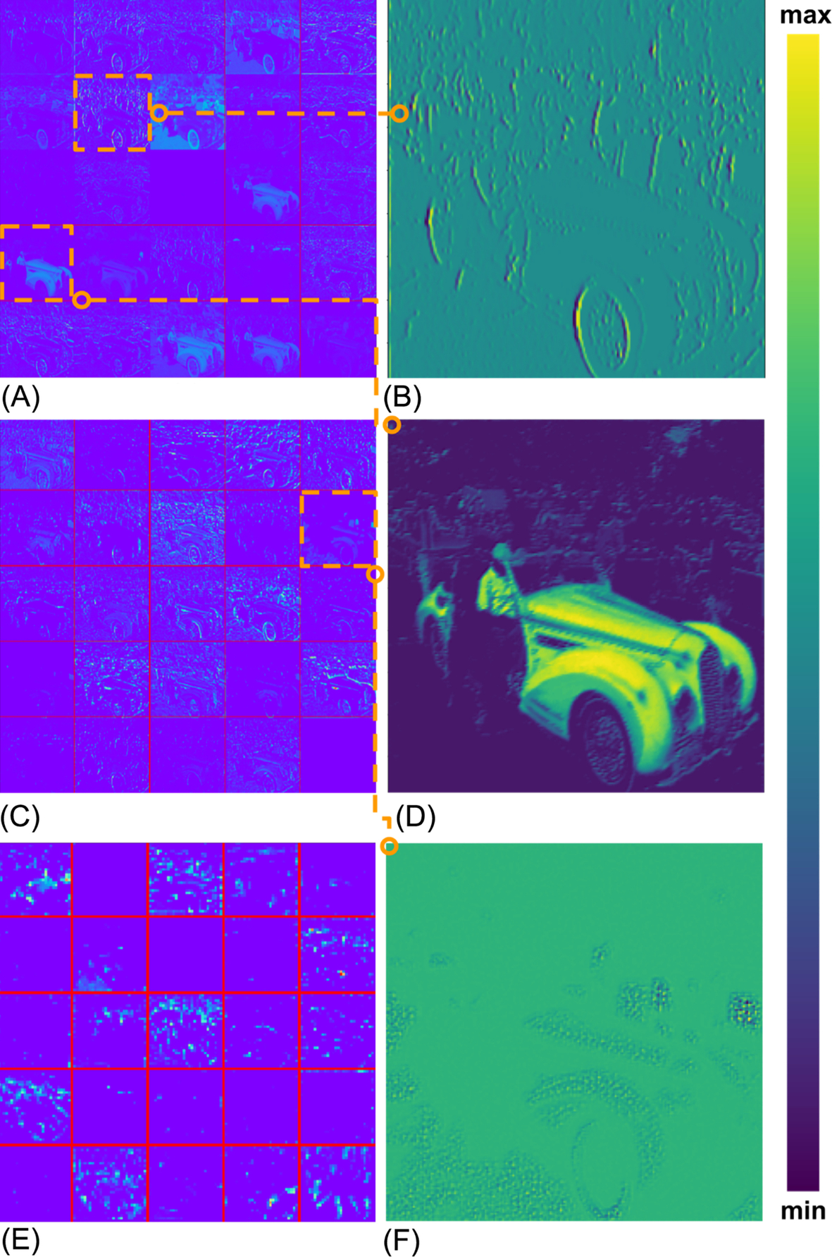
We have already discussed a feature extraction step in Section 4.7. All these features can be fed into NNs as well. What is interesting is that we can feed NNs with whole images, audio files, text series, etc., and let the NN learn features on its own. This is especially the case for CNNs where we can clearly see that filters are being learned in each convolutional layer. For example, in the first layer we can distinguish basic edge filters, blobs, corners, etc. In higher layers we can observe geometrical concepts (e.g., circles, squares) followed by others such as eyes, heads, hands, and wheels. In the last layers we can observe filters having high activations for entire objects (e.g., human, car, dog, cat, etc.). There is huge value in this because the NN can learn its own features based on the domain of a given task. It also usually outperforms handcrafted approaches (Fig. 27):


This code example of 2D convolution is a naive implementation. In a real deep-learning framework there will be a lot of different functions implementing convolution to better harness HW-specific operations and caches and using a faster algorithm based on parameters such as input size, kernel size, and number of inputs. One optimization is to modify the input matrix in such a way that convolution can be computed as a single matrix product. Another common technique is computing convolution as a multiplication in the Fourier domain, after appropriate padding (to prevent circular convolution). Usually, a developer doesn't have to implement any of these functions because they are usually done automatically within the deep-learning framework.
8.4.4 Convolutional Neural Network Classifier Example
Let’s now look at how to use PyTorch [29] (a deep-learning framework—we discuss other frameworks in Section 8.6) to train our own image classification. Our goal will be to classify images from the CIFAR-10 data set (as we’ve already described it in Section 4.6). In this example we won’t do the real heavy lifting. The data set is relatively small as is the neural net. A regular notebook or desktop PC without GPU should make it possible to complete the training within 10–20 min. It is also possible to use GPU clouds. Many companies provide some trial credit (e.g., Google Cloud Platform). While speaking about Google at the time of writing they also provide a service called Colab [30], where some GPU resources are available for free:

First, we need to import all the necessary modules (lines 1–9). The two main packages we are using are torch (PyTorch) and torchvision—utilities that make deep learning for computer vision even easier. Then we set out our neural net definition. Our net class is inherited from nn.Module and must employ the forward method. In constructor __init__ all building blocks are defined. Let us first look at the forward method that defines what our architecture will look like (see also Fig. 29). We have two blocks that are basically the same (lines 23–24)—a convolution layer followed by an activation function (relu) and then by pooling. On line 25 data are just transformed (flattened) from 4D (batch, height, width, channels) to 2D (batch, vector). This is necessary because on lines 26–27 a fully connected layer is used that expects input from only the 1D vector. Fully connected layers are followed by the relu activation function.

As we now know what our network should look like we can better understand the constructor. On line 14 the first convolution layer is defined. It expects 3 channels on its input. It has 8 filters (kernels) and the kernel size is 3 × 3. On line 15 a 2 × 2 max pooling layer is defined (it will reduce the size of feature channels by two as it divides each channel into 2 × 2 blocks and returns the maximum value from these four). On line 16 a second 3 × 3 convolution layer is defined. It expects 8 channels on the input and returns 16 channels. The kernel size is 3 × 3. On lines 18–20 fully connected layers are defined. They are defined by the number of input neurons and the number of output neurons. In this case we need to compute how many neurons there will be on the input. This depends on all previous layers and the input size. We know for sure that there will be 16 channels. Their resolution is affected by input size (32 × 32). The first 3 × 3 convolution without padding is applied, which means the filter size will be 30 × 30. Then max pooling is applied resulting in a size of 15 × 15. On top of that, a second 3 × 3 convolution without padding is applied, which means the filter size is 13 × 13. Max pooling is once again applied, thus making the filter size 6 × 6. Thus the input of the first fully connected layer will be 16 × 6 × 6 (see line 18). The number of output neurons (in our case 100) is a design choice. The last fully connected layer (line 20) must have 10 output neurons (as we have 10 classes).
On line 108 the loss function is chosen. In this case we are using cross-entropy loss ![]() , where N is number of classes (in our case 10), yi is the predicted probability of class i, and
, where N is number of classes (in our case 10), yi is the predicted probability of class i, and ![]() is 1 when the ith class is the correct one. A perfect model would have zero loss. But this won’t happen in practice. If you have zero loss you are either terribly overfitted or something is broken.
is 1 when the ith class is the correct one. A perfect model would have zero loss. But this won’t happen in practice. If you have zero loss you are either terribly overfitted or something is broken.
On line 109 an optimizer is defined. We are using a stochastic gradient descent (SGD) of learning rate of 0.1 and momentum of 0.9. A learning rate of 0.1 is pretty high (we are quite aggressive on training speed). If training diverges and loss starts to dramatically increase it might be time to consider learning rate reduction. As mentioned before, learning rate is an important hyperparameter.
The rest of the code is self-explanatory. Lines 79, 80 might be worthy of mention—where a data augmentation is added by doing random crop and horizontal flip (think why vertical flip wouldn’t be such a good idea for our case).


Even with this simple NN we were able to achieve a validation accuracy slightly above 60% (60.69%) after 20 epochs. To start building intuition we suggest the reader does the following exercises:
- • Try training without augmentation. What do you expect will happen?
- • Try to experiment with architecture (add more convolution layers) and add padding.
- • Try to experiment with optimizer parameters or try different optimizers (e.g., Adam).
8.4.5 Transfer Learning
It didn’t take long for the deep-learning community to discover that when we are short of training data it is possible to start from a pretrained model used to solve a similar problem. For example, if you want to classify dog breeds, you can start with a network trained to classify breeds of cats. It is common to start from pretrained general classifiers (e.g., ImageNet) and modify only the last layer or layers of the network (changing the number of classes). This concept works surprisingly well because the lower layers of the network have learned to detect basic entities such as edges, corners, and blobs, while later layers detect ears, eyes, wheels, etc. Further into the network the next layers detect even higher concepts such as head and leg. Subsequent layers lead to detection of complete concepts such as a human, dog, and car. Ultimately, the network can “see” the relationships between concepts. So when we need to distinguish between dog breeds we can still use trained kernels for eye detection, ear detection, etc. We only need to tune the last layers (or the last couple of layers depending on the tasks, intuition, and a trial-and-error approach).
8.5 Recurrent Neural Networks
The recurrent neural network (RNN), discovered by John Hopfield in 1982, is used for operations on sequences (e.g., text, voice). It enables NNs to learn patterns over time (e.g., detecting actions in video sequences, speech detection in audio, etc.). RNNs use a connection from their output to their input to allow the NN to gain a concept of temporal memory. This can be imagined as copying the whole NN and adding the same architecture into the new structure, and then sharing weights (see Fig. 30). The RNN can send some signals/states based on what was already processed on the input.

Building on RNNs there is an improved concept called long short-term memory (LSTM). Such networks allow speech applications to be improved dramatically (they are also widely used for text processing like machine translation). LSTMs were also successfully used in combination with CNNs for image captioning [31]. It’s also common to combine CNNs with LSTMs for video streams for tracking or events detection (Fig. 31).

8.6 Deep-Learning Frameworks
Which framework to choose? That’s the question. There are multiple possibilities and new ones are added each year. If asked to name the most common we would come up with TensorFlow [32], Caffe [33], and PyTorch [29].
TensorFlow (TF) is backed by Google. It is definitely the most used. It has a huge community and a fork called TensorFlow Lite focusing on mobile devices. Caffe seems to be in a decline. It was one of the first, widely used frameworks for CNNs.
PyTorch is a great tool for experiments. Compared with TensorFlow it is much easier to use to debug NN (as it boasts dynamic computational graph creation) and is commonly used in research. CNTDK is backed by Microsoft. The author’s personal suggestion is to design, tune, and debug NNs in PyTorch as it is simply easier. When dealing with performance issues try a move to TF (maybe even TensorFlow Lite).
There are also projects such as ONNX (Open Neural Network Exchange Format) [34] or NNEF (Neural Network Exchange Format, backed by Khronos) [35] that provide tools for NN interchange between different deep-learning frameworks. Currently, they work fine for mainstream DNN frameworks and ordinary NNs but might struggle when more complex layers are used.
9 What Is Necessary to Bring ML to the Edge?
Back in the day ML was heavily academic driven, where the primary goal was to make it work and push the boundaries of what was possible, no matter the cost. Engineers today have a completely different approach, especially in embedded application development where the industry is working to make its products smarter—but there are challenges:
- • Limited memory footprint—For example, in the previous section we introduced a brief history of ImageNet. Even more advanced models than AlexNet (which has around 60 M parameters, which if represented as float32 have a size of 240 MB) don’t have a negligible number of parameters nor a negligible memory footprint.
- • Limited computational resources—During the model-training phase large computational clusters powered by cutting edge NVIDIA GPUs are usually used (e.g., the relatively affordable NVIDIA GTX 1080 Ti has 11.3 TFLOPs, which means it can process 11.3 × 10¹² float operations per second). For example, MobileNet_v1_1.0_224 [36] needs 569 MACs/inference (MAC stands for multiply-accumulate operations). Therefore, there is clearly room for performance improvement if, for example, we switch from float to integer computations. Furthermore, switching from float to integer is essential because some devices don’t have a floating-point unit.
- • Power efficiency—Energy consumption is firmly linked to the number of calculations and use of memory and there is usually great interest in its reduction.
There’s an important observation that needs to be made when it comes to managing resources—when using fully connected (FC) layers in a neural network’s architecture usually a lot of memory space is consumed; on the other hand, convolutional layers are usually not as big but require significant computations. This suggests that optimization techniques may vary based on which layer is being optimized.
There are two main approaches to reducing a network’s size. The first and most commonly applied relates to reducing representative precision. One option is called quantization (e.g., going from float32 representation of weights down to int8 or lower). Low-rank factorization is another option; this is where matrices/tensors are approximated with smaller ones that are used for computations before they are reconstructed back into the original format. If necessary, it is possible to further compress the model’s size by applying encoding (e.g., Huffman encoding). The second approach is focused on making changes in architectures either by designing much smaller and/or computationally efficient NNs from the beginning or pruning NNs after or during a training phase. The use of these techniques is not exclusive, but they come into their own when used in combination to shrink the size and speed up inference. In addition, most techniques have a selectable degree of compression and thus can sacrifice some accuracy to meet given size/speed limits. The following sections discuss these techniques in more detail.
9.1 Quantization
The most important technique in the NN optimization domain is quantization [37]. Quantization does not change the architecture, instead it decreases the precision of weights and/or the activation functions. Most commonly seen is a decrease from float32 to int8 fixed-point precision—this alone reduces the memory footprint 4 ×. Note that for int8 multiplication you still need int32 registers.
The quantization of weights only reduces the size and might have no effect on inference time, although there’s a possible speedup because size reduction leads to the model fitting better into faster memory/caches, and depending on the HW it might also be computed faster doing computations in INTs instead of FLOATs. To improve performance the quantization of activations is also necessary. Usually, weights and activations are represented using 8 bit, but if there is a bias term (like in a convolutional layer) it is usually represented using 32 bit.
9.2 Pruning
Pruning neural networks is not a new concept. Papers such as Lecun et al. “Optimal Brain Damage” [38] date back to 1990. Pruning assumes, as many results show, that neural networks are overparametrized and thus there is redundancy. Moreover, some neurons do not contribute significantly. There might also be “dead neurons” with outputs that are always zero resulting from too high a learning rate in combination with activation functions prone to this behavior. If we find a way to rank the neurons based on how much they contribute, we can then decide to remove the less valuable ones to save space and potentially speed it up.
Ranking can be done according to either the L1/L2 norm of their weights, the neurons mean activations on some reasonable validation data set, the number of times a neuron wasn’t zero on a validation dataset, and other methods. After the pruning process accuracy drop is expected. The following step is commonly used to fine-tune the network to give the NN an opportunity to recover.
Speedup though is not guaranteed. Pruning usually results in irregular network connections that not only demand extra representation efforts, but also do not fit well with parallel computation. This is usually worthwhile only when NN size is the issue or it results in an NN with high sparsity, where overhead from sparse matrix computation is negligible. Another possibility is structured pruning [39] (e.g., removing whole convolution kernels, etc.).
9.3 Postprocessing vs. Dynamic Optimization
Back in the day, researchers tried the most straightforward approach—take a trained network, prune it, quantize weights, and see what happens. Even if this was done carefully, it was very frequently followed by a huge accuracy drop. Today, what is usually done is either fine-tuning or training where the pruning is scheduled, say, to start at the 50th epoch, and quantization is also added in the end. These techniques usually prolong the training phase but provide smaller and more computationally/energy-efficient NNs without a dramatic drop in accuracy.
Another important observation for optimization, which might seem counterintuitive, is that starting with an optimized NN (quantized, pruned, and low-rank approximation applied) and training it from scratch doesn’t usually work. It either ends up with poor accuracy (compared with an overparametrized NN) or it doesn’t converge at all. These results are more observational since there are is no proper theory supporting these processes yet.
9.4 Low-Rank Factorization
The key idea behind low-rank factorization is to replace matrix multiplications with more matrix multiplications. Sounds counterintuitive, right? The reason this works is that these new matrices are smaller. The number of operations during matrix multiplication AB, AϵRM × N, BϵRN × O is MNO multiplications and M(N − 1)O additions. For simplicity let’s take it as just MNO multiply-accumulation operations (MACs).
A well-known matrix decomposition method is singular value decomposition (SVD). A = UΣV∗, UϵRM × M, ΣϵRM × N, VϵRN × N. Σ is a diagonal matrix, and diagonal entries are called singular values. By construction these singular values can be placed in descending order. The compression technique is based on the fact that we can take only the first k singular values, thus reducing matrix sizes into UϵRM × k, ΣϵRk × k, VϵRk × N. The magic happens when we do matrix multiplication: UΣVB. We start with VB, which is kNO MACs, and end up with matrix DϵRk × O. We can have UΣ precomputed as matrix CϵRM × k, then the CD multiplication will cost MkO MACs. The whole UΣVB with UΣ precomputed cost is kNO + MkO = kO(N + M).
Consider the last fully connected layer of VGG [16]. It has an input size of 4096 and an output size of 1000. What happens here is Wx + b,WϵR1000 × 4096, xϵR4096 × 1, bϵR1000 × 1, where W is the weight matrix, x is input, and b is the bias term. When W is decomposed a reasonable k is chosen. For k = 800 there is almost zero gain because the original multiplication will cost 4.096 M MACs, and with decomposition it will be 4.076 M. For k = 400 we need only 2.038 M MACs—a 2 × savings. The memory requirements will also be smaller. From NM (4.096 M) weights going down to kN + kM (for k = 400; it is the same as 2.038 M MACs). The reason memory is the same as MACs is that we are multiplying by a vector, thus O = 1.
This approach is good to follow as it has a fine-tuning phase compensating for a possible drop in accuracy. In the end one FC layer will be replaced by two smaller layers. The first has an input size of 4096, an output size of k, and no bias term. The second layer has an input size of k, an output size of 1000, and a bias term b.
Other techniques take this idea even further. There are more optimal approaches than SVD—a good example is Fastfood kernel decomposition [40, 41]. It is applied only to matrix multiplications. When we speak about convolution we are dealing with tensor multiplication (tensor is a more general concept than matrices and vectors). 4D tensor multiplication usually takes place in convolution. Similar to SVD decomposition are Tucker decomposition [42] and CP decomposition [43]. However, they take place in the higher dimensional space used for NN compression.
9.5 Architecture Design
As is known, fully connected layers consume a lot of memory, but convolutions stress the processing resources. Another way to save resources is to design the architecture with optimality in mind. In the field of CNNs there are networks, such as FD-MobileNet [44] and ShuffleNet [45], doing exactly this. One recent trend is not to use fully connected layers as they are prone to overfitting and have many parameters resulting in a big memory footprint.
There are several ideas related to convolution layers. Probably one of the first was published in [46]. This involved an NN architecture called SqueezeNet where 1 × 1 convolutional kernels are applied before more complex 3 × 3 convolution layers to reduce the number of input channels. The authors showed comparable accuracy with AlexNet, but with fewer parameters. At first sight 1 × 1 convolutional kernels might seem like a nonsense. What they do though is to combine feature maps in the linear way. Usually, an activation is applied on top of them adding more nonlinearity into the system.
Another idea is the depthwise-separable filter, which was introduced as part of the MobileNets architecture [36]. The trick is in dividing the standard convolution layer into two steps. Instead of doing N-times convolution on all input features (where N is the number of filters) a convolution is done only once followed then by N 1 × 1 convolutions to end up with N separate feature maps. For example, a 3 × 3 depthwise-separable convolution (as used in [36]) uses between eight and nine times less computation than standard convolutions with only a small reduction in accuracy.
For further reading we suggest a paper about SqueezeNext that focuses on hardware-aware NN design [47].
10 Edge Learning/Training
We have discussed ML on the edge only in terms of inference. But what about edge training as well? There might be some strong motivation such as privacy or connectivity (either connectivity is not present or has bandwidth limitations).
How do you update your NN on the edge? What if, for example, the number of classes in the network needs to change (e.g., a face recognition system where a new face is added). You could perform the training again from scratch, although this is probably not worth the effort nor even possible. Some approaches allow you to do a small portion of training—so-called fine-tuning—but this usually comes with issues like overfitting to new examples.
The most commonly used approach is to use an NN as a feature extraction tool. We can do this by removing the last layer (usually softmax in the case of classification) and end up with some alternate output layer. With this application in mind we can intentionally design an architecture such that we have, for example, 128 neurons in the penultimate layer thus having a descriptor of 128 numbers. We can take these numbers as a feature descriptor and feed it into some lightweight ML algorithms such as SVM and k-NN.
Let’s look intuitively at how this approach works. Consider that the last layer was fully connected with softmax activation. This means one dot product plus a nonlinearity function have been used to properly classify the output of the penultimate layer. Therefore, when we train a classifier on top of the penultimate layer we have the same expressive power, but the training of, say, SVM is much faster and easier to do than retraining the whole NN.
Another frequently used technique is to freeze most of the layers and just fine-tune the remaining layers (e.g., last layer) on a small data sample. However, it is important to remember that we must restrict ourselves to inference when it comes to NN deployment, but when we need to carry out training we need to support efficient computation of backpropagation, which complicates things a lot. Currently, most edge inference engines don’t support training.
Other more advanced approaches are built on top of concepts like k-shot learning [48] [49]. This is a hot research area in which new classes are learned based only on k examples, where k is a small number (sometimes even 1).
Bringing ML to the edge is not an easy task, but the potential impact on improving or creating so far unimaginable products is enormous. An increase in the number of research projects on these topics would greatly help to do this as would a number of open-source projects and raising embedded community interest. As stated at the beginning of this chapter this field is changing each day. We should expect thrilling times in the future when embedded learning meets machine learning.