
Introduction to Dynamic Risk Analyses
Warren D. Seider*,1; Ankur Pariyani†; Ulku G. Oktem*,†; Ian Moskowitz‡; Jeffrey E. Arbogast‡; Masoud Soroush§ * University of Pennsylvania, Philadelphia, PA, United States
† Near-Miss Management LLC, Philadelphia, PA, United States
‡ American Air Liquide, Newark, DE, United States
§ Drexel University, Philadelphia, PA, United States
1 Corresponding author: email address: [email protected]
Abstract
This chapter places recent advances in dynamic risk analyses in perspective. After some preliminary concepts such as alarms, near misses, and accidents, conventional risk analysis approaches are reviewed. Next, the use of Bayesian analysis in dynamic risk analysis without alarm data is discussed. This leads to dynamic risk analysis with extensive alarm data and a review of typical safety systems and upset states. Data compaction approaches needed to compact data associated with thousands of daily alarm events are presented. For a large fluidized-bed catalytic conversion unit, the use of Bayesian analysis with copulas to estimate safety system failure probabilities (and the probabilities of plant trips and accidents) is demonstrated. Next, using plant and operator data, methods for creating informed prior distributions for Bayesian analyses are covered. These methods are shown to improve the risk analyses for an industrial steam-methane reformer. Throughout, concepts are reviewed, covering the basics and referring the reader to more complete presentations in the original papers. This chapter is intended for process engineers and operators concerned with safety risks, who seek to learn and implement methods of quantitative dynamic risk analysis.
Keywords
Risk; Safety; Bayesian analysis; Prior distributions; Alarms; Event trees; Data compaction; Operator response times
1 Introductory Concepts and Chapter Objectives
Automated control and safety systems are prevalent in modern chemical plants, as they help plants return to normal operating conditions when abnormal events occur. The databases associated with these systems contain a wealth of information about near miss occurrences. Frequent statistical analyses of the information can help identify problems and prevent accidents and expensive shutdowns. Such analyses are referred to as dynamic risk analyses.
Predictive maintenance is an important evolution in the effective and efficient management of industrial chemical processes. Often predictive maintenance is focused upon individual equipment within a process (e.g., compressors). Lately, in addition, proactive risk management is recognized as a key concept for the evolution to the next level of safety, operability, and reliability performance in chemical operations involving plant-wide analyses toward prescriptive maintenance. Dynamic risk analysis refers to a methodology that utilizes various tools to help collectively to achieve proactive risk management. Hence, its application has been gaining significant importance in the chemical and process industries.
This chapter discusses dynamic risk analysis of alarm data. It provides a general overview of what these analyses are, how they can be used in chemical processing to improve safety, and challenges that must be addressed over the next 5–10 years. It also highlights current research in this area and offers perspectives on methodologies most likely to succeed.
1.1 Alarms, Near Misses, and Accidents
Fig. 1 is a generic control chart for a primary process variable (P), which is divided into three zones: green-belt, yellow-belt, and red-belt. An abnormal event occurs when a process variable leaves its normal operating range (green-belt zone), which triggers an alarm indicating transition into the yellow-belt zone. If the variable continues to move away from its normal range, the variable may transition into its red-belt zone, indicated by second-level alarm (e.g., LL, HH) activation. Once a variable remains in its red-belt zone for a prespecified length of time (typically on the order of seconds), an interlock activates and an automatic shutdown occurs. If the automatic shutdown is unsuccessful, an accident would occur if not prevented by physical protections (e.g., pressure relief devices, containment).
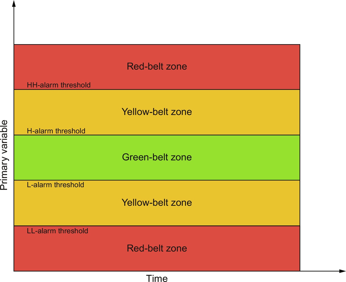
The accidents are rare, high-consequence (e.g., significant human health, environmental, and/or economic impact) events. The costs of unplanned shutdowns—which happen infrequently, but not rarely—are also quite significant. Of course, the layers of protection in place are usually successful, and therefore, the vast majority of abnormal events are arrested before accidents occur. When an abnormal event is stopped and the variable returns to its green-belt zone, this is considered a process near miss event (which is simply referred to as a near miss in this chapter). Accidents are typically preceded by several near misses, as the latter are higher-probability, lower-consequence events. As a result, vast amounts of near miss data can be extracted from alarm activations for dynamic risk analyses. Depending on their criticality, abnormal events can be classified into different categories (Pariyani, Seider, Oktem, & Soroush, 2010). In this chapter, the following two categories are used: least-critical abnormal events that cross the high/low alarm thresholds, but do not cross the high–high/low–low alarm thresholds, and most-critical abnormal events that cross the high–high/low–low thresholds, often associated with interlock systems or emergency shutdown (ESD) systems.
Many companies record these alarm occurrences in databases and operators, engineers, and managers seek guidance from these databases by evaluating various key performance indicators (see alarm management standards published by ANSI/ISA 18.2 (2009) and EEMUA (2007)) and paying attention when special events such as alarm flooding and chattering occur (Kondaveeti, Izadi, Shah, Shook, & Kadali, 2010). Most of the time, further analysis is done after process upsets, unanticipated trips, and accidents occur.
Companies are becoming increasingly aware that these alarm databases are rich in information related to near misses. In recent years, researchers have been developing key performance indicators, or metrics, associated with potential trips (shutdowns with no associated personal injury, equipment damage, or significant environmental problem) and accidents; leading indicators (i.e., events or trends indicating the times these trips and accidents are likely to occur); and probabilities of failure of the individual safety systems and the occurrence of trips and accidents (ANSI/ISA 18.2, 2009; EEMUA, 2007; Khan, Rathnayaka, & Ahmed, 2015; Pariyani et al., 2010; Villa, Paltrinieri, Khan, & Cozzani, 2016; Ye, Liu, Fei, & Liang, 2009). When conducted at frequent intervals, the analyses that are associated with these performance indicators are often referred to as dynamic risk analyses or, simply, near miss analyses.
1.2 Conventional Risk Analyses
Risk assessment is an important component of the US Occupational Safety and Health Administration's (OSHA) process safety management (PSM) standard, which includes (among other elements) inherently safer design, hazard identification, risk assessment, consequence modeling and evaluation, auditing, and inspection. PSM has become a popular and effective approach to maintain and improve the safety, operability, and productivity of plant operations. As part of this, several risk assessment methods have been developed.
The use of quantitative risk analysis (QRA), which was pioneered in the nuclear industry in the 1960s, was extended to the chemical industry in the late 1970s and early 1980s after major accidents such as the 1974 Flixborough explosion in the UK and the 1984 Bhopal incident in India. Chemical process quantitative risk analysis (CPQRA) was introduced as a safety assessment tool by the AIChE's Center for Chemical Process Safety (CCPS) in the 1990s as a means to evaluate potential risks when qualitative methods are inadequate. CPQRA is used to identify incident scenarios and evaluate their risk by defining the probability of failure, the various consequences, and the potential impacts of those consequences. This method typically relies on historical data, including chemical process and equipment data, and human reliability data to identify hazards and risk-reduction strategies. A recent review article by Khan et al. (2015) examines qualitative, semiquantitative, and quantitative methods developed in the past 10–15 years. Much emphasis is shifting toward quantitative techniques involving fault trees, event trees, and bowtie networks to understand better safety events. This quantification empowers plant managers and operators to make decisions based upon their current risk assessment. In offshore drilling, bowtie models have been used to represent the potential accident scenarios, their causes, and the associated consequences (Abimbola, Khan, & Khakzad, 2014; Khakzad, Khan, & Amyotte, 2013a, 2013b). These involve dynamic risk analysis using Bayesian statistics.
Other risk assessment methods were subsequently developed to analyze industry-wide incident databases (Anand et al., 2006; CCPS, 1999; Elliott, Wang, Lowe, & Kleindorfer, 2004; Kleindorfer et al., 2003; Meel et al., 2007). These databases include: CCPS's Process Safety Incident Database (CCPS, 1999, 2007) which tracks, pools, and shares process safety incident information among participating companies; the Risk Management Plan database, RMP*Info (Kleindorfer et al., 2003), developed by the US Environmental Protection Agency (EPA); the National Response Center (NRC) database, an online tool set-up by NRC to allow users to submit and share incident reports; and the Major Accident-Reporting System (MARS), which is maintained by the Major Accident Hazards Bureau (MAHB). Recent risk analyses associated with chemical plant safety and operability have used Bayesian statistics to incorporate expert opinion (Meel & Seider, 2006; Valle, 2009; Yang, Rogers, & Mannan, 2010), and fuzzy logic to account for knowledge uncertainty and data imprecision (Ferdous, Khan, Veitch, & Amyotte, 2009; Markowski, Mannan, & Bigowszewska, 2009). Such methods have significantly improved quantitative risk assessment.
While these methods have been important in quantifying safety performance, a large amount of precursor information pointing to unsafe conditions has been overlooked and unutilized, because it resides in large alarm databases associated with the distributed control system (DCS) and ESD system (also referred to as “alarm data”). The alarms help plant operators assess and control plant performance, especially in the face of potential safety and product-quality problems. The alarm data, therefore, contain information on the progression of disturbances and the performance of regulating and protection systems. However, despite advances in alarm management standards and procedures, alarm data analysis methods reported in the literature quantify only performance, not risk. Risk is qualitatively inferred from these qualitative performance metrics (e.g., alarm frequency).
Several comprehensive algorithms and software packages to evaluate process safety risks with an eye toward developing and implementing appropriate protective measures have been developed over the last 2 decades (Risk World, 2013; Vinnem, 2010). Most of these systems rely on accident and failure databases mentioned above, which provide information such as accident frequencies, consequences, and associated economic losses, to perform QRAs. Other tools, discussed later, utilize a quantitative methodology for the risk analysis either in real time or on-demand, but they do not focus on estimating the likelihood of incidents or the failure of safety systems. The analyses that involve accidents and failures only, and exclude day-to-day alarm information and associated near miss data, are not highly predictive. They overlook the progression of events leading up to near misses—information that can only be found by analyzing data found in alarm databases.
A study of an ammonia storage facility conducted by the Joint Research Center and Denmark Risk National Laboratory of the European Commission (Lauridsen, Kozine, Markert, & Amendola, 2002) found that risk estimates based on generic databases of reliability and failure data for commonly used equipment and instruments are prone to biases, providing widely varying results depending on data sources.
For these reasons, the importance of utilizing process-specific databases for risk analyses has been gaining recognition. The next section discusses dynamic risk analysis methods and how they extract valuable risk information not available from conventional risk analyses.
1.3 Dynamic Risk Analysis
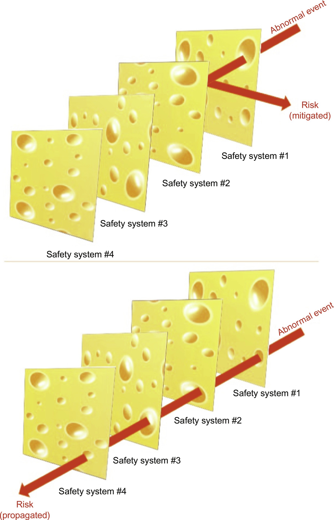
Accidents are rare events, occurrence of which is often described using the popular Swiss-cheese model (Reason, 1990). In this model, each layer of protection (safety system) is considered as a layer (slice) of Swiss cheese, with the holes in the slice (varying in size and placement) corresponding to weaknesses in the layer of protection (Fig. 2), and safety systems of a process are represented by several layers (slices) of Swiss cheese lined up in a row. According to this model, failures occur when the holes in the individual slices line up, creating trajectories of accident opportunities. This model accounts for the element of chance that is involved in the occurrence of failures.
Reports of major accident investigations often list several observable near misses—i.e., less-severe events, conditions, and consequences that occur before the accident. Regular, thorough analysis of process near misses could prevent the emergence of risky conditions from being overlooked.
On the basis of the sensitivity and importance, certain plant variables are labeled as primary variables—denoted by pP, p for primary and P for process variable (typically temperature, pressure, flow rate, …). These variables are closely related to process safety and are associated with the interlock system. When these variables move beyond their interlock limits, ESDs or “trips” are triggered, often after a small time delay. The remaining variables in the plant are referred to as secondary variables, which are not associated with the interlock system—and denoted by sP, s for primary and P for process variable. For large-scale processes, typically thousands of variables are monitored; however, only a small percentage (less than 1%–10%) are chosen as primary variables. The primary variables are selected during the design and commissioning of plants by carrying out analyses of tradeoffs between the safety and profitability of the plant. Note that the control chart described in Fig. 1 is for a primary variable. For secondary variables, similar control charts exist, however, they do not have red-belt zones. As a result, they can indicate only least-critical abnormal events. Also note that, for many processes, control charts are provided for quality variables (typically, viscosity, density, average molecular weight, …)—denoted by pQ, p for primary and Q for quality variable, and sQ, for secondary quality variables. See Pariyani, Seider, Oktem, and Soroush (2012a) for more complete coverage involving quality variables.
Although the layers of protection are designed to keep process (and quality) variables within acceptable limits, the chemical processes frequently encounter special causes (i.e., sudden or unexpected causes of variations in process conditions due to unexpected phenomena), resulting in abnormal events. An event-tree corresponding to a primary variable's transition between belt zones (in response to an abnormal event) is shown in Fig. 3. The first-level (e.g., L, H) alarm system activates safety system 1 (SS1), which is typically an operator action. When SS1 is successful, with probability 1−x1, continued operation (CO) is achieved, as indicated by path P1. The second-level (e.g., LL, HH) alarm system activates SS2, which is typically a more aggressive operator action. When successful, with probability 1−x2, near miss CO is achieved, indicated by path P2. If the primary variable occupies the red-belt zone for a predetermined length of time (on the order of seconds), SS3, the automatic interlock system for plant shutdown, will become activated. The interlock system is designed to be independent of alarm systems, and the activation of SS3 is determined by an independent set of sensors. It should be noted that if the interlock system is designed to have no delay time the probability of SS2 success is equal to zero (x2=1) since the operator has precisely no time to respond for such a design. If SS3 succeeds, with probability 1−x3, the interlock shutdown occurs and an accident is avoided, represented by path P3. If the interlock shutdown is unsuccessful, an accident occurs at the plant, represented by path P4. With a proper design, x3 should be very small consistent with the specified safety integrity level (SIL). Since the interlock system is independent of the alarm system, the success of SS3 does not depend on factors such as operator skill and alarm sensor faults. However, it can be concluded that if either SS1 or SS2 is successful in arresting the special-cause event (SCE), the activation of the interlock system is avoided altogether. In some cases, alarms are officially considered as a layer of protection and contribute to the SIL rating of the overall safety system, composed of SS1, SS2, and SS3. Therefore, herein alarms are included in the safety systems—noting that often the full alarm system is not considered part of a plant's SIS. In this systematic way, the success and failure of each safety system, along with its associated process consequence, is tracked. See Section 2.5 for a more complete discussion of event trees and their paths.
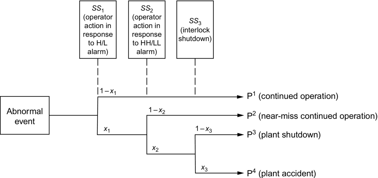
The probability of each consequence can be calculated when the safety system failure probabilities are known; e.g., the probability of a plant shutdown is:
These consequence probabilities are important to process engineers and plant managers, who seek to maintain very high probabilities of continued safe operation with quantifiably very low probabilities of potential plant shutdowns and accidents. The failure probabilities associated with operator action, x1, and in many cases x2, are often difficult to estimate. A manufacturing process typically has control systems that can mitigate most disturbances, with few propagated to SCEs. And, when few historical data are available, especially for SS2, and the failure probabilities of higher-level alarm and safety interlock systems, x1, x2, and x3 estimated from historical data alone have very high uncertainties, not providing useful predictive capabilities (Gelman, Carlin, Stern, & Rubin, 2014). Therefore, there is a need for a method of estimating the failure probabilities from process and alarm data along with our knowledge of the process dynamics and operators’ behavior (Jones, Kirchsteiger, & Bjerke, 1999; Mannan, O'Connor, & West, 1999).
In industrial practice, methods such as HAZOP and HAZAN (Crowl & Louvar, 2011; Kletz, 1992) are commonly utilized to make safety and reliability estimates of processes on a unit-operation basis. Equipment–failure probabilities estimated from statistical and equipment–manufacturer data are used to estimate process failure probabilities. But, more recently, dynamic risk analyses have been employed to update these equipment–failure probabilities as real-time data are measured.
This chapter traces the development of dynamic risk analysis over the past 2 decades. First, Yi and Bier (1998) introduced the techniques to use consequence data to estimate dynamically the failure probabilities of safety systems. They used copulas to improve the estimates of failure probabilities of rare events (shutdowns and accidents). Meel and Seider (2006) then extended these methods for a hypothetical plant involving an exothermic continuous stirred tank reactor (CSTR). Pariyani et al. (2012a) and Pariyani, Seider, Oktem, and Soroush (2012b) extended Meel and Seider (2006) using alarm consequence data, and showed the performance of their methods by calculating the failure probabilities of a fluidized catalytic cracking unit. Kalantarnia, Khan, and Hawboldt (2009) and Kalantarnia, Khan, and Hawboldt (2010) conducted further work on dynamic risk analysis and proposed improved consequence assessment approaches using Bayesian-based failure mechanisms. Khan et al. (2015) and Villa et al. (2016) provided a literature review of risk assessment approaches over the last 2 decades, including dynamic risk analysis. More recently, Moskowitz, Seider, Soroush, Oktem, and Arbogast (2015) and Moskowitz et al. (2016) proposed a method of improving process models and introduced new probabilistic models that describe SCE occurrences and operator response times, allowing for estimating alarm and safety system failure probabilities more accurately.
1.4 Bayesian Analysis
Bayesian analysis is often used to determine the failure probabilities of alarm and safety interlock systems. The central dogma of Bayesian analysis is that parameters of probability distributions (e.g., mean and variance) are themselves distributions. Unlike classical statistics that seeks to capture the true moments of a distribution, Bayesian statistics acknowledges that the moments of a distribution may not be fixed, and seeks to estimate the probability distributions of the moments. This analysis often requires significantly fewer data to make meaningful predictions (Berger, 2013; Gelman et al., 2014). Additionally, as the process dynamics and operators’ behavior change with time (because of factors such as process unit degradation and operators’ improved skills), real-time data can be collected and used to estimate more accurate failure probabilities in real time.
Bayesian analysis is a statistical approach to reasoning under uncertainty, which is briefly reviewed in this section, as applied to the estimation of failure probabilities. The principal steps in the application of Bayesian analysis include: (i) specifying a probability model for unknown parameter values that includes prior knowledge about the parameters, if available; (ii) updating knowledge about the unknown parameters by conditioning this probability model using observed data; and (iii) evaluating the goodness of the conditioned model with respect to the data and the sensitivity of the conclusions to the assumptions in the probability model.
The uncertainty of the failure probability of a safety system, x, is modeled using a probability distribution function, f(x), called the prior distribution. Historical data and/or insights (e.g., based on experience) can then be used to obtain an improved failure probability distribution, f(x|Data), called the posterior distribution using the Bayes theorem:
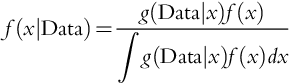
where g(Data|x) is the distribution of identically and independently distributed (i.i.d.) data conditional upon x, which is called the likelihood function.
1.4.1 Prior Distributions
In many cases, a prior distribution is approximated by a distribution from a convenient family of distributions, which when combined with the likelihood function gives a posterior distribution in the same family. In this case, the family of the prior distribution is a family of conjugate priors to its likelihood family distribution. For example, the Beta distribution is a family of conjugate priors to the Bernoulli distribution. Consider the following Beta distribution as the prior distribution for a random variable, x:
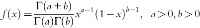
where the Gamma function is:
The expected value and variance of x, denoted by E(x) and Var(x), are:
For this Beta distribution, Meel and Seider (2006) assumed the data belong to the Bernoulli family, and derived the posterior distribution, utilizing Bernoulli's likelihood function and the Beta prior distribution.
Values of the parameters of the prior distribution function, a and b, can be obtained using historical information, or expert knowledge. In the absence of such information, a noninformative (often flat) prior distribution is utilized that weighs all of the parameters equally; e.g., a uniform distribution.
2 Dynamic Risk Analysis Using Alarm Data
Dynamic risk analysis using alarm databases was first introduced by Pariyani et al. (2012a, 2012b) to identify problems and correct them before they result in sizable product and economic losses, injuries, or fatalities. In most industrial processes, vast amounts of alarm data are recorded in their DCSs and ESD systems. The dynamic risk analysis method involves the following steps:
1. Track abnormal events using raw alarm data.
2. Create event trees that show all of the possible paths an abnormal event can take when propagating through the safety systems.
3. Use a set-theoretic framework, such as that developed by Pariyani et al. (2012a) to compact the data into a concise representation of multisets.
4. Perform a Bayesian analysis to estimate the failure probabilities of each safety system, the probability of trips, and the probability of accidents (Pariyani et al., 2012b).
Steps 1–3 are presented in the subsection that follows in which the event trees and set-theoretic formulations allow compaction of massive numbers (millions) of abnormal events. For each abnormal event, associated with a process variable, its path through the safety systems designed to return its variable to the normal operation range is recorded. Event trees, as shown in Fig. 3, are prepared to record the successes and failures of each operation, with on the order of 106 paths through event trees stored. As introduced herein, and shown in (Pariyani et al., 2012a), the set-theoretic structure condenses the paths to a single compact data record, leading to significant improvement in the efficiency of the probabilistic calculations and permitting Bayesian analysis of large alarm databases in real time. The latter is in Step 4, which was introduced in Section 1.4.
2.1 Typical Alarm Data
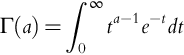
Alarm data are normally comprised of alarm identity tags for the variables, alarm types (low, high, high–high, etc.), times at which the variables cross their alarm thresholds (in both directions), and variable priorities. The associated interlock data, which is of greater consequence, contains trip event data, timer-alert data, and so on. A screenshot of a typical alarm log file for a brief period is shown in Fig. 4. Every row represents a new entry, associated with a process (or quality) variable. Column A displays the times in chronological order, with each entry displaying the “Year–Month–Day Hour: Minute a.m./p.m.” Column B indicates the entry type: alarm, change in controller settings, and so on. Column C shows the alarm tag of the variable (defined during the commissioning of the unit). Column D shows the alarm type [LO (low), LL (low–low), HI (high), and so on.]. Column E shows the drift status of the alarms, either ALM (alarm) or RTN (return); that is, whether the variable drifts beyond or returns within the alarm thresholds. Column F shows the alarm priority, and column G presents a brief description of the alarm. Similar data entries exist for the interlock data.
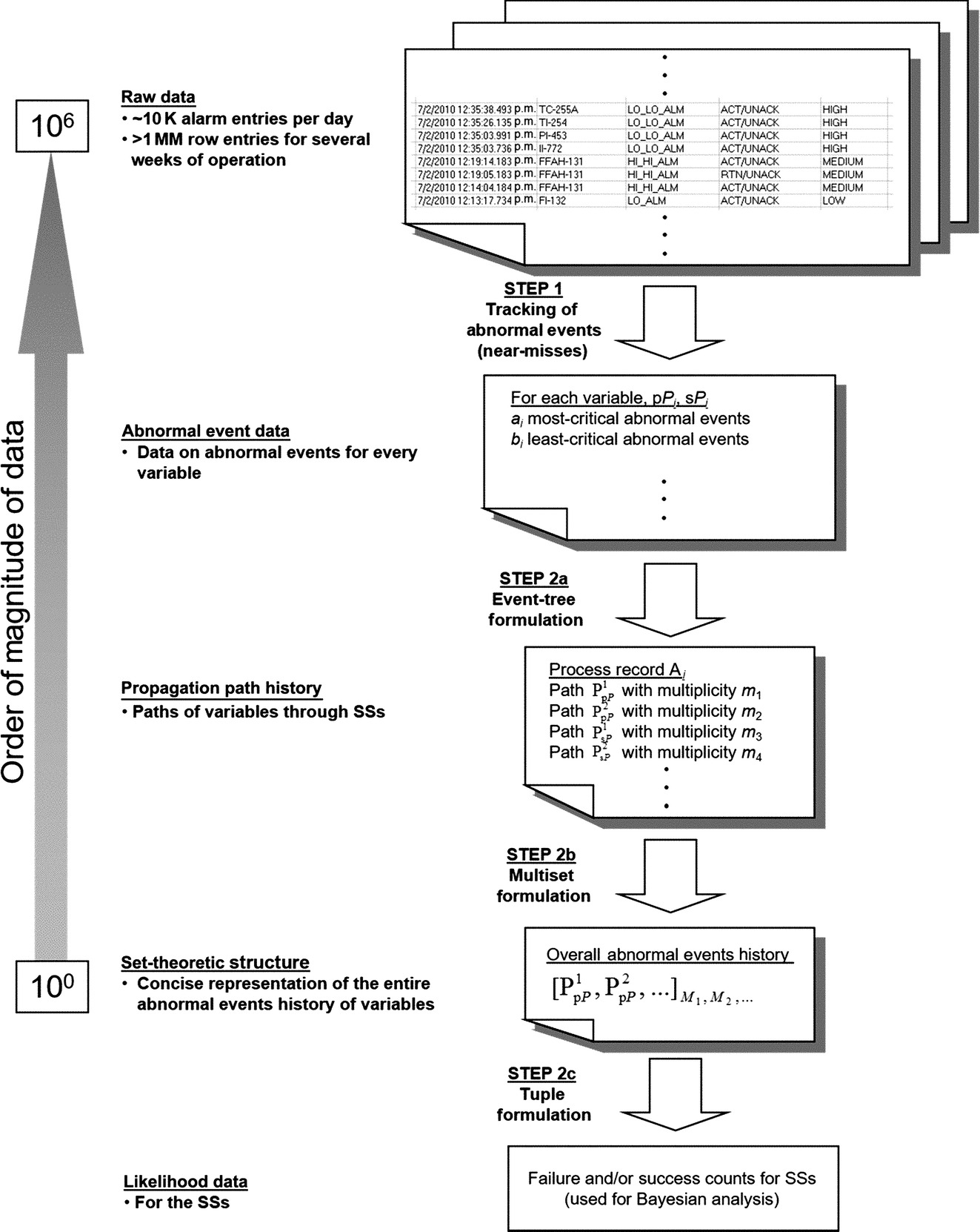
In some industrial-scale processing plants, 5000–10,000 alarm activations may realistically occur daily, with on the order of 106 alarm activations over a few months. To carry out Bayesian analysis, it is required to create a compact representation of this big data. Fig. 5 shows a schematic of the steps to create the compact representation, beginning with the raw data at the top and, after the steps described herein, resulting in likelihood data required for Bayesian analysis to estimate the failure probabilities of the safety systems.
2.2 Safety Systems
Next, returning to the discussion of safety systems in Section 1.3, three of the most commonly used systems are further described, noting that the number of systems and their functionalities are dependent on the specific chemical plants.
Operator (machine+human) corrective actions, Level I—SS1—which refers to human operator-assisted control to keep the variables within their high/low alarm thresholds and to return them to normal operating conditions. When unsuccessful, variables enter into their red-belt zones.
Operator (machine+human) corrective actions, Level II—SS2—which refers to human operator-assisted control to keep the variables within their high–high/low–low alarm thresholds and to return them to normal operating conditions. These corrective actions are more rigorous than those for level I, because when unsuccessful, the interlocks are activated, often after a short time delay.
Interlock shutdown—SS3—which refers to an automatic, independent, ESD system that shuts down the unit (or part of the unit).
To assess the reliability of these systems for a process, a framework involving event-trees and multisets is outlined in this section to provide a compact representation of vast alarm data, which facilitates the statistical analysis using Bayesian theory. The combined framework accounts for the complex interactions that occur between the DCS, human operators, and the interlock system—yielding enhanced estimates and predictions of the failure probabilities of the safety systems and, more importantly, the probabilities of the occurrence of shutdowns and accidents. This causative relationship between the SSs is modeled using copulas (multivariate functions that represent the dependencies among the systems using correlation coefficients).
2.3 Upset States
A process is said to be in an upset state when process variables move out of their green-belt zones, indicating “out-of-control” or “perturbed” operation. Upset states lead to deterioration in operability, and safety performances of the process. Equations to estimate the operability and safety performances have been proposed in the literature (Pariyani et al., 2010; Ye et al., 2009). The following two upset states are presented here, with additional details available (Pariyani et al., 2010).
Operability upset state (OUS), where at least one of the secondary process variables lies outside its green-belt zone, but all the primary process variables lie within their green-belt zones. In this case, the operability performance deteriorates significantly, whereas safety performance appears to be maintained. This occurs, for example, when the flow rate of a stream (a secondary process variable) moves just above its green-belt zone, but not sufficiently far to move the primary process variables out of their green-belt zones.
Safety upset state (SUS), where at least one of the primary process variables lies outside its green-belt zone. In this case, both safety and operability performances are affected and automatic action is required unless the plant operator takes effective corrective action.
Clearly, plants can move from one upset state to another as disturbances (or special causes, which cause abnormal events) progress.
2.4 Principal Steps in Dynamic Risk Assessment—Summary
The dynamic risk assessment method herein consists of three steps, shown as three regions of the pyramid in Fig. 6. The steps are: (1) near miss tracking, (2) event-tree and set-theoretic formulation, and (3) Bayesian analysis.
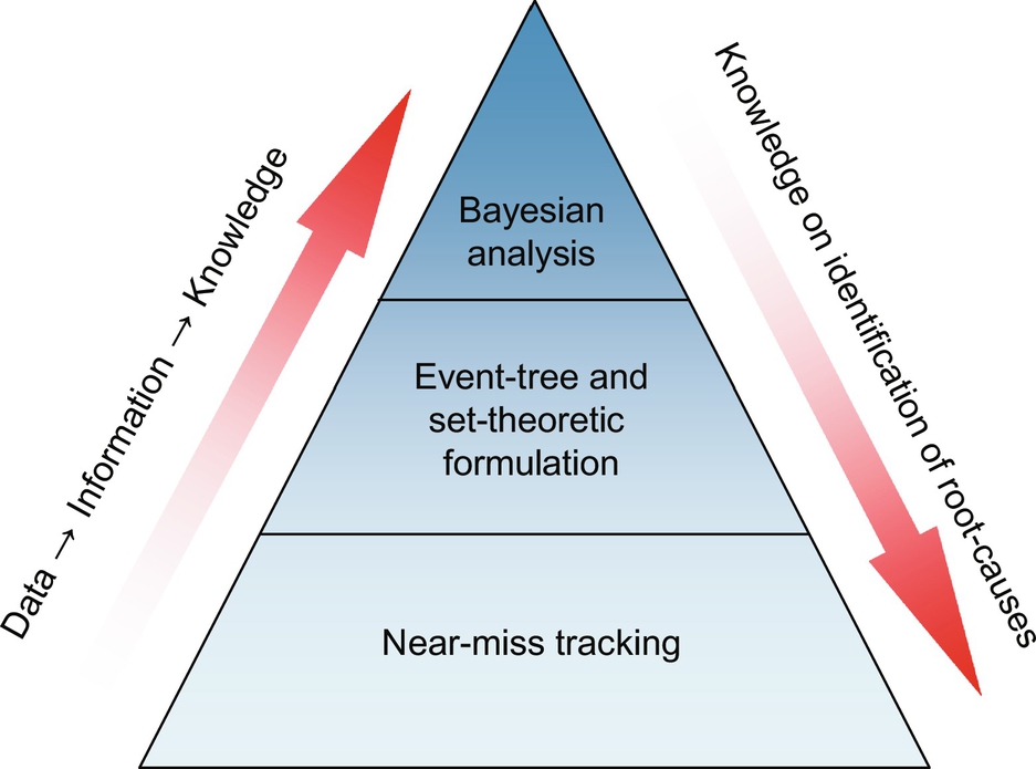
Near Miss Tracking refers to identification and tracking of near misses over an extended period of time (weeks, months, and so on). As mentioned earlier, the abnormal events experienced by the process variables are recognized as near misses. Pariyani et al. (2010) presented techniques for tracking abnormal events and analyzing recovery times to quantify, characterize, and track near misses experienced by individual and groups of variables over different periods of time. Using Pareto charts and alarm frequency diagrams, these techniques permit identification of variables that experience excessive numbers of abnormal events, drawing the attention of plant management to potential improvements in control strategies, alarm thresholds, and process designs. They also suggest opportunities to explore the root cause(s) of each abnormal event and reduce the frequency of each abnormal event. These approaches improve upon alarm management techniques by drawing attention to the severity of abnormal events experienced by variables and their associated recovery times (rather than alarm counts only). The results suggest the need to carry out these statistical analyses in real- or near-real time—to summarize for plant operators those alarms associated with the most abnormal events and requiring the most attention; that is, allowing prioritization of the numerous flags raised by the alarms.
Event-tree and set-theoretic formulation permits the transformation of near miss data to information on the performances of the safety systems. As presented in the discussion of Fig. 5, in this step, the near miss data that tracks: (a) abnormal events, (b) the propagation of abnormal events, and (c) the attainment of end states, is stored in set-theoretic formulations to represent the branches of event-trees.
As abnormal events arise in processes, they are handled by the SSs, whose actions guide the process variables through their green-, yellow-, and red-belt zones, resulting in either continued normal operation (variables in their green-belt zones) or upset states (OUS, SUS). The sequences of responses (that is, successes or failures) of the SSs are the paths (denoted by Pi) followed by the process variables and are described by the branches of the event-trees, as shown in Fig. 3. They track abnormal events to their end states (i.e., normal operation, plant shutdown, accident, and so on). Using a generalized set-theoretic formulation (discussed in Section 2.5.3), these paths are represented in a condensed format—to facilitate Bayesian analysis. Stated differently, near miss data extracted from the alarm data show how variables move among their yellow- and red-belt zones to their end states. From these, event-trees are created and represented with new set-theoretic notations. This permits the systematic utilization of the historical alarm databases in Bayesian calculations to estimate failure probabilities, the probabilities of accidents, and the like.
Bayesian analysis refers to the utilization of the transformed data to obtain knowledge (that is, statistical estimates) of the performances (in terms of failure probabilities) and pair-wise interaction coefficients of the safety systems. Also, the probabilities of incidents are estimated. These estimates help to identify the root-causes in the process, for example, the SSs with high failure probabilities or variables experiencing high abnormal event rates. In particular, consider a case when the failure probabilities of the operator corrective actions (SS1 and SS2) are high—giving operators and managers incentives to identify their root-causes—possibly due to insufficient operator training, stress factors, and so on.
2.5 Data Compaction
2.5.1 Objectives
When compacting millions of alarm data entrees, Pariyani et al. (2012a) introduced path formulations to trace the process variables together with a set-theoretic formulation. This section presents these two formulations.
2.5.2 Event-Tree Formulations for Process (and Quality) Variables
The event-tree formulations depict the actions of the safety systems (SSs) as they respond to abnormal events—with their branches representing the paths traced by the process (and quality) variables. Note that each SS is represented by a node, with the success or failure of each system denoted by S or F, respectively, along two branches leaving each node.
Fig. 3 shows an event-tree for an abnormal event (when a primary variable leaves its green-belt zone). The tree is illustrated for the three typical SSs discussed earlier. Again, primary process variables are denoted by pP and secondary process variables by sP (and primary and secondary quality variables are denoted by pQ and sQ).
Depending on the performance (success or failure) of these SSs, four paths are possible—with two paths leading to continued operation, CO (when variables return to their green-belt zones), one path leading to emergency shutdown, ESD (when a primary variable enters its red-belt zone and interlock is activated), and one path leading to plant accident (when the SSs fail to remove a primary variable from its red-belt zone). The latter often leads to loss of life, serious injuries, and major equipment losses, involving major economic losses due to product losses and manpower requirements to return the process to normal operation.
The paths are numbered according to the index of the end state in the event-tree—from top to bottom, using the notation, PpPi where i is the path counter. The primary variables follow the uppermost path, PpP1, when the basic process control system (BPCS) fails to keep them within their green-belt zones resulting in least-critical abnormal events, but the SS1 successfully returns them to their green-belt zones. Symbolically, the path is represented by SpP1 or simply S1, where SpPk or simply Sk denotes the success of safety system k. Also, the combined path and its end state are denoted as PpP1-CO.
The primary variables follow the second path, PpP2, when they enter their red-belt zones, marking the failure of SS1, indicating the first level of corrective actions by operators. However, the second-level (more rigorous) corrective actions by the operators successfully return them to their green-belt zones. This path, is represented by ![]() , where Fk denotes the failure of SSk. Together with its end state, this most-critical abnormal event is denoted as PpP2-CO. The primary process variables follow the third path, PpP3, when they enter their red-belt zones, marking the failures of operator corrective actions (both levels) indicated by SS1 and SS2 and successful actions by the interlock, indicated by SS3, resulting in a shutdown. This path is represented by
, where Fk denotes the failure of SSk. Together with its end state, this most-critical abnormal event is denoted as PpP2-CO. The primary process variables follow the third path, PpP3, when they enter their red-belt zones, marking the failures of operator corrective actions (both levels) indicated by SS1 and SS2 and successful actions by the interlock, indicated by SS3, resulting in a shutdown. This path is represented by ![]() . Together with its end state, this most-critical abnormal event is denoted as PpP3-ESD.
. Together with its end state, this most-critical abnormal event is denoted as PpP3-ESD.
The primary variables follow the fourth path, PpP4, when the interlock fails to remove the variables from their red-belt zones or bring plant operations to a shutdown, resulting in a plant accident. This path is represented by ![]() . Together with its end state, this most-critical abnormal event is denoted as PpP4-ACCIDENT.
. Together with its end state, this most-critical abnormal event is denoted as PpP4-ACCIDENT.
At times, variables oscillate between their yellow- and red-belt zones, before returning to their green-belt zones. In such cases, the above notation applies—with the criticality of the abnormal events determined by the highest belt zone entered. This concise notation, with the set-theoretic representation in the next subsection, has been shown to represent effectively complex alarm sequences for the Bayesian analysis. As an example, consider an abnormal event with a process variable (assuming no interlock activation): (a) entering its red-belt zone, (b) returning briefly to its yellow-belt zone, (c) reentering its red-belt zone, and (d) returning to its green-belt zone. For this abnormal event, the SS1 failed to keep the variable within its yellow-belt zone, and the SS2 succeeded, in its second attempt, in returning the variable to its green-belt zone. Note that, in practice, when variables experience oscillations about their thresholds, deadbands (of 2%–5%) are often applied to prevent nuisance alarms (Kondaveeti et al., 2010).
For variables (and processes) involving different schemes of SSs, the notation remains applicable. For example, if the interlock system (SS3) is designed to be activated without any time delay (indicating absence of SS2) for a primary variable, only three paths are possible—with their end states, denoted as: PpP1-CO, PpP3(-II)-ESD, and PpP4(-II)-ACCIDENT. In this notation, the path numbers are unchanged and the event-trees remain applicable when certain SSs are not included.
In practice, the interlock system is associated only with critical variables of the process (primary variables) to reduce costly shutdowns. The remaining secondary variables involve only corrective actions by the operators to return them to their green-belt zones. Using the earlier steps, event-trees can be constructed for secondary variables (sPs) that enter their yellow- or red-belt zones (without any interlock actions).
Note that if one or more primary variables enter their red-belt zones, corrective actions taken by SSs are likely to return them and, in turn, the secondary variables to their green-belt zones. Because of interactions between the primary and secondary variables, the effects of their corrective actions are channeled to the latter, causing them to return to their green-belt zones as well. However, the recovery times of pPs and sPs often vary significantly. These interdependent effects due to nonlinear interactions can be handled effectively by implementing multivariable, nonlinear model-predictive controllers (MPCs). Herein, the event-trees do not explicitly account for the auxiliary effects of SSs on different categories of variables. Also, these event-trees are applicable to only continuous processes, wherein process variables return to their green-belt zones eventually (except when shutdowns or accidents occur). Event trees for batch processes can be developed similarly, with time-varying thresholds. Finally, returning to Fig. 5, in Step 1, abnormal events in the raw alarm data are tracked to extract abnormal event histories for each variable, pPi, sPi—involving most- and least-critical abnormal events.
2.5.3 Set-Theoretic Formulation—Case Study 1
To introduce the set-theoretic formulation, consider Case Study 1, which is presented in Table 1 as a process report for a typical continuous process over a brief period (consisting of minute-by-minute status updates in which a disturbance drives a few process variables out of their green-belt zones). Between 1:00 and 1:01 p.m., the process enters an OUS. In the next 2 min, it moves from an OUS to a SUS as four of its primary process variables move out of their green-belt zones. However, within the next minute, all the variables are returned to their normal operating ranges, with CO occurring—thanks to levels I and II corrective actions by the operators.
Table 1
Process Report—Case Study
| 1:00 p.m. | Normal operation |
| 1:01 p.m. | Four primary variables pP1, pP2, pP3 and pP4, enter their yellow-belt zones (4 high alarms go off) |
| 1:02 p.m. | The first primary variable, pP1, enters its red-belt zone (1 high–high alarm goes off) |
| 1:03 p.m. | Operators successfully diagnose and correct the problem, with four process variables returned to their green-belt zones |
In this case study, four abnormal events (three least-critical and one most-critical) occurred, after the BPCS failed to keep its process variables within their green-belt zones. As the SSs responded, pP2, pP3, and pP4, which entered their yellow-belt zones only, followed the path, S1, whereas, the first primary process variable, pP1, which entered its yellow- and red-belt zones, followed the path ![]() . Thus, based on the event-tree in Fig. 3, two distinct paths were followed: (a) PpP1—followed by pP2, pP3, and pP4 and (b) PpP2—followed by pP1—all leading to the end state, CO. Thus, this abnormal events history, which shows several variables experiencing abnormal events over a period of time, is represented by a collection of paths, traced by the variables, leading to the same end state, and therefore, is referred to as a process record. Note that an abnormal events history may include more than one process record, corresponding to different end states attained by the variables; e.g., CO, plant shutdown, etc.
. Thus, based on the event-tree in Fig. 3, two distinct paths were followed: (a) PpP1—followed by pP2, pP3, and pP4 and (b) PpP2—followed by pP1—all leading to the end state, CO. Thus, this abnormal events history, which shows several variables experiencing abnormal events over a period of time, is represented by a collection of paths, traced by the variables, leading to the same end state, and therefore, is referred to as a process record. Note that an abnormal events history may include more than one process record, corresponding to different end states attained by the variables; e.g., CO, plant shutdown, etc.
Again, returning to Fig. 5, using the abnormal event data created in Step 1, propagation paths through the SSs are extracted in Step 2a using the event-tree formulations discussed earlier. Note that for the process report in Table 1, a process record is created comprised of paths PpP1 and PpP2, followed m1 (=3) and m2 (=1) times by the four variables.
Next, the key premises of the set-theoretic model are presented:
(1) The paths followed by the variables are modeled as n-tuples, where n-tuples are ordered lists of finite length, n. Like sets and multisets (discussed later), tuples contain objects, as discussed by Moschovakis (2006). However, the latter appear in a certain order (which differentiate them from multisets) and an object can appear more than once (which differentiates them from sets). Herein, for paths of event-trees, modeled as n-tuples, n denotes the number of SSs, and the objects are Boolean variables with permissible values, 0 (FALSE) and 1 (TRUE), for the failure and success of the SSs, respectively. When any system is not activated, a null value, φ, is used. For the event-trees discussed earlier, the paths are modeled as three-tuples (for the three SSs), given by:
This notation is also applicable to event-trees with fewer SSs. For example, the three-tuple notation for PpP3(-II) and PpP4(-II) are (0, φ, 1) and (0, φ, 0).
(2) The set of distinct paths, that is, {PpP1, PpP2} for Case Study 1, denoted as am, followed by the process variables is referred as an underlying set of paths. Note that because the elements in a set cannot be repeated (Moschovakis, 2006), the four paths (for four abnormal events) for Case Study 1 are not explicitly shown. To include the number of abnormal events associated with each path, multisets (Blizard, 1991) are used herein. In a multiset, the elements are repeated with a multiplicity equal to the number of repetitions; and the cardinality of the multiset is the sum of the multiplicities of its elements. Note that a set is a multiset with unique elements. Hence, the abnormal events history in the process report in Table 1 is represented as a process record, Am, represented using a multiset of cardinality 4, [PpP1, PpP1, PpP1, PpP2], or in the standard format for multisets, [PpP1,PpP2]3,1, where the multiplicities of PpP1 and PpP2 are 3, and 1, respectively, with an associated CO end state.
It follows that, using the event-tree and set-theoretic formulation herein, any abnormal events history, comprised of abnormal events involving different process variables, can be represented as process records; that is, multisets of paths (modeled as three-tuples herein) traced by the process variables as the SSs take actions. Also, for any process record, a unique and nonempty underlying set of paths is defined; whose elements are the various paths of the event-trees, as discussed earlier.
Returning to Fig. 5, in Step 2b, the overall abnormal events history is summarized as a multiset of paths. The second block from the bottom shows a multiset, for the entire alarm database, showing typical paths, PpP1 and PpP2, and their multiplicities, M1 and M2. Finally, in Step 2c, the likelihood data for the safety systems are obtained from the overall abnormal events history using a tuple formulation, as illustrated for a fluidized catalytic cracking unit next. These contain the failure and/or success counts to be used in Bayesian analysis.
2.5.4 Set-Theoretic Formulation—FCCU Case Study
In this case study, alarm data over an extended time period, associated with a fluid-catalytic-cracking unit (FCCU) at a major petroleum refinery that processes over 250,000 barrels of oil per day, are used. The unit has on the order of 150–200 alarmed variables and as many as 5000–10,000 alarm occurrences per day—indicating 500–1000 abnormal events daily. A total of 2545 abnormal events occurred for the primary variables during the study period. The abnormal events history of the primary variables for the study period is summarized in Table 3 of Pariyani et al. (2012a)—demonstrating that the new set-theoretic framework provides a compact representation in handling thousands of abnormal events depicting success/failure paths followed by the process variables through the SSs. This framework facilitates the Bayesian analysis to compute failure probabilities of the SSs and incident probabilities.
2.6 Bayesian Analysis Using Copulas
As discussed by Pariyani et al. (2012b), significant interactions between the performances of the SSs, measured as failure probabilities, are due to nonlinear relationships between the variables and behavior-based factors. In their Bayesian analysis, they use copulas to account for these interactions.
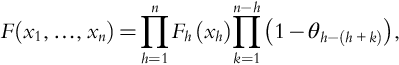
To introduce copulas, the Sklar (1973) shows that a copula function can model the cumulative joint distribution, F(x1, …, xn), between random variables when the correlation between them is unknown:
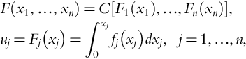
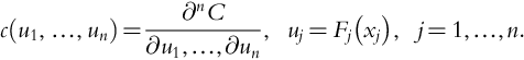
where C is the copula function, and F1, …, Fn denote the marginal cumulative distributions for random variables, x1, …, xn, respectively. The joint distribution is independent of the type of random variable and only depends upon the degree of correlation. Similarly, the joint distribution, f(x1, …, xn), can be obtained as a function of the copula density, c, and the marginal distributions (f1, …, fn):
where c is defined as:
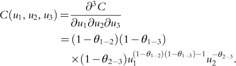
Several multidimensional copula families have been reported (Nelsen, 1999; Yi & Bier, 1998), one of which is the Cuadras and Auge copula:
where θj−q expresses the degree of correlation between the random variables xj and xq, and ![]() when n−h=0. In three dimensions, Eq. (6) becomes:
when n−h=0. In three dimensions, Eq. (6) becomes:
and the copula density (Eq. 6) is:
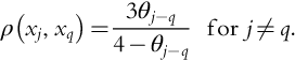
Spearman's ρ-rank correlation coefficients are often used to represent the degree of correlation in joint distributions using copulas. These are a function of the copula alone and are independent of the marginal distributions of the correlated random variables. Many copulas have closed-form expressions for the ρ-rank correlation coefficients as a function of their correlating parameters, as discussed by Nelsen (1999); for example, the ρ-rank correlation coefficient, ρ(xj, xq), and the correlation parameters θj−q, in the Cuadras and Auge copula, are related by:
To understand the usage of the Cuadras and Auges copula to estimate the failure probabilities, the reader is referred to Meel and Seider (2006). In that paper, four Bayesian models are implemented for the same CSTR consequence data, each model differing in the use of the Cuadras and Auges copula. Therein, prior joint distributions for safety systems are expressed using the copula density in Eq. (5). The failure probabilities of various safety systems (associated with the CSTR) are updated in real time, and the reader gains an appreciation for the dependency of these probabilities on the copula structure. Also, matrices are provided to specify the ρ-rank correlation coefficients that represent the interactions between the failure probabilities associated with safety systems. Finally, the parameters of the Beta prior distributions and the resulting posterior distributions are provided. These latter distributions depend on the actions of the prior safety systems in the event-tree.
2.6.1 FCCU Results
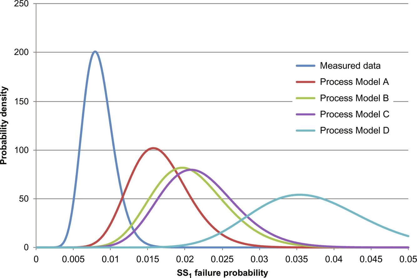
For the FCCU, Pariyani et al. (2012b) use the Normal and Cuadras and Auges copulas. Unfortunately, due to space limitations, the detailed correlation matrix and discussion are not included herein, as well as the details of the prior distributions. Instead, results are shown in Fig. 7 for the failure probabilities of the SSs.
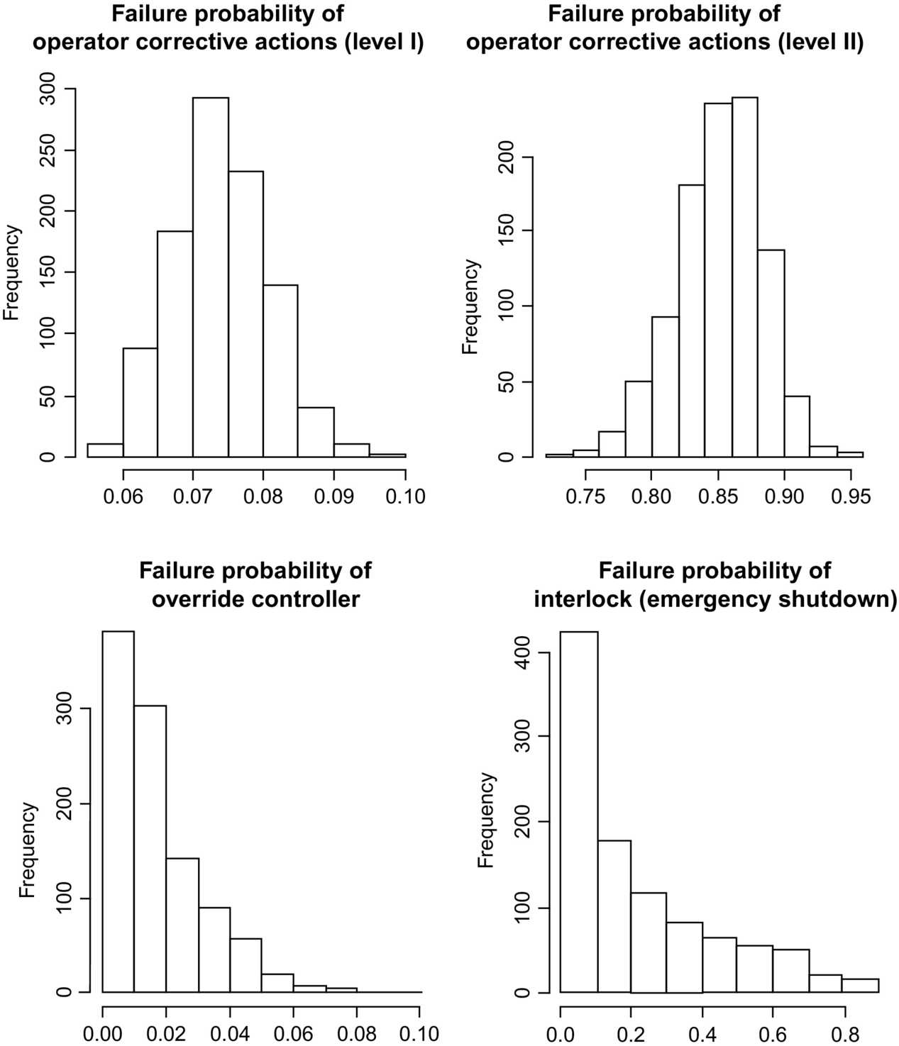
The mean posterior failure probability (and associated variance) of the operator's level I corrective actions is fairly low (=0.074)—indicating their robust performance. However, for operator's level II corrective actions, the mean failure probability is high (=0.851), indicating their difficulties in keeping the variables within their orange-belt zones—note they use an additional safety system (referred as override controller) with an additional orange-belt zone between the yellow- and red-belt zones. Stated differently, the probability that the primary variable moves from its yellow-belt zone to its orange-belt zone is just 7.4%, while the probability of moving from its orange-belt zone to its red-belt zone is 85%—indicating ineffective actions of level II operator corrections. Hence, for the FCCU, to prevent variables from moving to their red-belt zones, it is important to prevent their crossing into orange-belt zones.
The mean failure probability of the override controller is also quite low (=0.017). However, its variance is high, as compared to that of previous safety systems. Also, the failure probability of the ESD system is relatively uncertain, due to the availability of few data points. In these cases, past performances (over several months and years) and/or expert knowledge regarding their failures (often supported by system test results), are desirable. The latter can be derived from the dynamic risk analysis of near miss data from related plants. Note that similar results can be obtained for individual time periods.
3 Informed Prior Distributions
Next, techniques for constructing informed prior distributions when carrying out Bayesian analyses to determine the failure probabilities of safety systems are presented (Moskowitz et al., 2016, 2015). This is to circumvent the inaccuracies introduced because rare-event data are sparse having high-variance likelihood distributions. When these are combined with typical high-variance prior distributions, the resulting posterior distributions naturally have high variances preventing reliable failure probability predictions. As discussed in this section, the techniques use a repeated-simulation method to construct informed prior distributions having smaller variances, which in turn lead to lower variances and more reliable predictions of the failure probabilities of alarm and safety interlock systems.
3.1 Constructing Informed Prior Distributions
The method involves the eight steps listed in Table 2. In Steps 1–3, a robust, dynamic, first-principles model of the process incorporating the control, alarm and safety interlock systems, is built. The model can then be simulated using a simulator such as gPROMS v.3.6.1 (2014), which is used herein. The control system in the model mimics the actual plant control system, with consistent control logic and tuning. Likewise, the alarm and safety interlock systems in the model mimic those in the plant. For operator actions, this can be difficult, as operators often react differently to alarms. In particular, expert operators may take into account the state of the entire process when responding to alarms. When creating a model, the likelihood of operator actions must be considered. Either the modeler can use the action most commonly taken by operators or a stochastic simulation can be set-up in which the different actions are assigned probabilities.
Table 2
Steps to Construct an Informed Prior Distribution
1. Develop a dynamic first-principles process model
2. Incorporate control system into the dynamic process model
3. Incorporate the alarm and safety interlock system into the dynamic process model
4. Postulate potential special-cause events to be studied
5. For each special-cause event, construct a distribution for the event magnitudes, ASC (i.e., for a postulated pressure decrease, construct a probability distribution for a decreasing magnitude).
6. For each special-cause event, construct a distribution for operator response time, τ.
7. For each special-cause event, conduct the simulation study according to the algorithm described in Fig. 8 to simulate the range of possible event magnitudes, ASC, and operator response time, τ.

8. Using the method of Gelman et al. (2014), estimate parameters of a distribution model (e.g., Beta distribution) representing the data generated in Step 7—this is used as an informed prior distribution.
With these models, SCEs are postulated in Step 4. The list of SCEs can be developed from various sources: HAZOP or LOPA analysis, observed accidents in the plant (or a similar plant), near miss events at the plant (or in a similar plant), or from risks suggested in first-principles models of the plant. For each SCE, an event magnitude distribution is created in Step 5. A distribution for operator response time, τ, is created in Step 6. These three distributions are used along with the dynamic simulation in Step 7 to obtain simulation data. Lastly, in Step 8, the simulated data are used to regress parameters for the informed prior distribution. The algorithm used to generate simulation data (Step 7) and regresses informed prior distribution parameters (Step 8) is described in the paragraph below, and represented pictorially in Fig. 8.
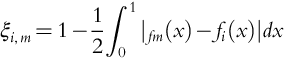
The script that manages the dynamic simulations starts by sampling A1 from the event magnitude distribution created in Step 5. Note that Fig. 8 shows a normal distribution centered at μSC with variance σSC2, however any distribution can be used. Assign the number of safety system failures, i, to i=0. With this A1, the user script samples τ1 from the distributions created in Step 6. Although Fig. 8 shows uniform distributions (with the maximum operator response time at τmax), any distribution can be used. With A1 and τ1, a dynamic simulation is run. If the safety system fails to avoid a plant-wide shutdown, then i=i+1; if the safety system is successful, i is not incremented. When n<N, n=n+1; i.e., for sampled Ai and τi, a dynamic simulation is run, and i is adjusted when necessary. After N iterations, j1=i/N is calculated, in the range [0, 1]. Then m is incremented and Am sampled, the inner loop is reexecuted, and jm is calculated. When the outer loop has been completed (m=M), a vector of M elements (j1, …, jM) has been accumulated. The average and variance of this vector are used to calculate α and β of the Beta distribution. Note that because the Beta distribution is the conjugate prior of the binomial likelihood distribution, it is the recommended choice. The number of simulations, M×N, is chosen, recognizing that more simulations yield a smaller prior distribution variance.
3.2 Testbed—Steam-Methane Reforming (SMR) Process
A typical SMR process is shown in Fig. 9. After pretreatment, natural gas feed (70) and steam (560) are mixed before entering the process tubes of an SMR unit (90), where hydrogen, carbon monoxide, and carbon dioxide are produced. This hot process gas (100) is then cooled and sent to a water–gas shift converter (110), where carbon monoxide and water are converted to hydrogen and carbon dioxide. The process gas effluent (120) is cooled in another heat exchanger, producing stream 170, which is sent to two water extractors. Note that the last section of this heat exchanger is used to transfer heat to a boiler feed water makeup stream in an adjacent process. The gaseous hydrogen, methane, carbon dioxide, and carbon monoxide, in stream 210, are sent to PSA beds. Here, high-purity hydrogen is produced (220), and the PSA-offgas is sent to a surge drum. Stream 800 from the surge drum is mixed with hot air (830) and a small amount of natural gas makeup (815), and sent to the furnace side, where it is combusted to provide heat to the highly endothermic process-side reactions. Its’ hot stack gas (840) is sent through an economizer, where it is used to heat steam (520), some of which are used on the process side (560), with the rest available for use or sale as a steam product (570).

In modeling for process safety, emphasis should be placed on units that present the greatest risk; i.e., have the largest probabilities of incidents multiplied by incident impact (Kalantarnia et al., 2009). In an SMR process, temperatures rise above 1300 K with pressures over 20 atm. Because overheating can lead to process-tube damage and failure, potentially leading to safety concerns, its model should receive special attention. In Moskowitz et al. (2015), partial differential and algebraic equations (PDAEs), that is, momentum, energy, and species balances, accounted for variations of pressure, temperature, and composition in the axial direction for both the process- and furnace-side gases. For the reforming tubes, the rigorous kinetic model of Xu and Froment (1989) was used, while the furnace–gas combustion reactions were modeled using a parabolic heat-release profile. Convection and radiation were modeled on the furnace side, where view factors were estimated using Monte Carlo simulations and gray–gas assumptions. The heat transfer on the process side was modeled by convection only, assuming a pseudo steady state between the process gas and catalyst. Details of the models are presented by Moskowitz et al. (2015).
The PSA beds represent a cyclic process, with beds switched from adsorption to regeneration on the order of every minute. This type of separation scheme induces oscillatory behavior throughout the SMR process. As the flow rates, compositions, and pressures fluctuate in effluent streams from the PSA beds, variables throughout the entire plant fluctuate as well. In processes with such cyclical units, buffer tanks are often used to dampen fluctuations. However, typical buffer-tank sizes (comparable to SMR-unit sizes) reduce the amplitude of these fluctuations by on the order of 50%. In Moskowitz et al. (2015), the SMR process test-bed involves four PSA beds, which operate in a four-mode scheme, with each bed undergoing adsorption, depressurization, desorption, and repressurization steps.
In the full safety process model used by Moskowitz et al. (2015), the SMR-unit and PSA-bed models are used in conjunction with dynamic models for the water–gas shift reactor, water extractor, surge tank, heat exchanger, and steam drum. Furthermore, the controls used with the dynamic process model are consistent with those used in the Air Liquide process. The full process is modeled using the software package, gPROMS. A challenging aspect of the full process model involves convergence of the PSA-offgas recycle loop. Note that this process model combines SMR and PSA-bed units within a plant-wide scheme with PSA-offgas recycle. The results computed by gPROMS are consistent with the process data from the industrial plant. This plant-wide model is extremely useful for building leading indicators and prior distributions of alarm and safety interlock system failure probabilities.
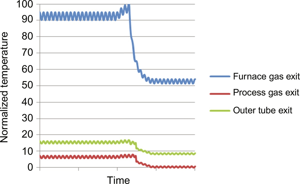
With this dynamic process model, process engineers can simulate SCEs and track variable trajectories. Consider an unmeasured 10% decrease in the Btu rating, due to a composition change of the natural gas feed (40), in Fig. 9. Note that the makeup stream (815) on the furnace side is relatively small and is not changed in the simulation. Initially, because the process stream contains less carbon, less H2 is produced. Because these reactions are endothermic, less heat from the furnace is consumed by the reactions and the furnace temperature rises, as shown in Fig. 10. Also, the process-side temperature increases. Eventually, the low-carbon PSA-offgas reaches the SMR furnace. With less methane for combustion, the furnace temperature decreases, as does the temperature of the process gas. This effect is shown in Fig. 6. Note that the temperatures oscillate due to the natural gas oscillation in stream 800 from the PSA-offgas surge tank—due to the cyclic nature of the PSA process.
3.3 SMR Informed Prior Distributions
For the SMR process in Fig. 9, a loss in steam pressure to the reformer side (stream 560), was simulated with the responses of the safety systems monitored (Moskowitz et al., 2015). For small disturbances, the process control system handled the effect of steam pressure decreases. There is a flow controller on the steam line, whose set point is generated using a linear equation involving the flow of natural gas into the SMR process side, seeking to achieve a constant steam-to-carbon ratio in the process tubes. This control system normally arrests typical fluctuations in steam pressure and flow rate, but for large steam pressure decreases, feedback control alone is insufficient. In this case, the control valve is wide open, with a flow rate insufficient to accompany natural gas fed to the SMR unit. For this reason, an investigation was undertaken to assess the effectiveness of the alarm systems associated with the SMR steam line. When the steam flow rate is below its L-alarm threshold, the steam-to-carbon ratio drops, accompanied by an increase in the process-side temperature and potential tube failure. Because of these operating limits, an interlock was placed at the HH-alarm threshold with a time delay. This time delay, of several seconds, reflects that the temperature threshold may be exceeded in this case for a short period of time and permits the operator to respond rapidly in an attempt to bring the furnace temperature below its HH-alarm threshold.
Three operator responses to the alarm are simulated: (1) the valve on the steam line is opened, (2) the valve on the makeup fuel line is pinched, and (3) the dampers associated with air flow in the furnace are opened (effectively increasing air flow rate). When the operator is able to bring the furnace temperature below the HH-threshold before the interlock delay times out, an automatic shutdown is avoided. If, however, the operator is unable to do so, the interlock is activated and a plant shutdown occurs. The simulated abnormal event leads to either a success of SS2 (interlock is avoided), or a failure of SS2 (interlock is activated). It is desirable to have a reliable estimate of x2, the probability that the operator is not successful, despite only a few activations of this HH-alarm during the recorded history over several years.
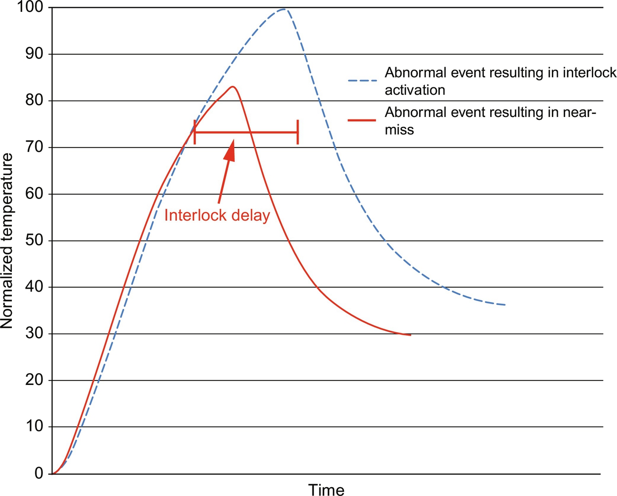
Herein, a pressure decrease in the steam line to the process side of the SMR unit was simulated. The magnitude of the pressure decrease was a random variable, sampled from a normal distribution centered at 50% of stream pressure. The response time of the operator was taken as a random variable, sampled from a uniform distribution ranging from 0 to 15 s. The operators three responses were all incorporated into the simulation as step changes in valve settings. One thousand simulations were run, and the effectiveness of the operator's response in each simulation was tracked. In some simulations, the operator successfully reduced the furnace temperature below the interlock threshold in the allotted time before the automatic shutdown. In others, the operator failed and the plant was shutdown. In Fig. 11, a temperature trajectories for events resulting in an interlock activation and in a near miss are shown. In the scenario where SS2 succeeds, the temperature is brought below the interlock threshold within the interlock delay time. Note that the action of the control system was observed early in the trajectory, but it was insufficient to avoid the abnormal event and eventual plant shutdown. The average number of safety system failures was recorded for the simulations, as well as the failure variance, which were used to generate a Beta distribution to describe the failure probabilities. The Beta distribution, which has just two parameters, was created easily and is supported only in the range [0, 1], which bounds the failure probability.
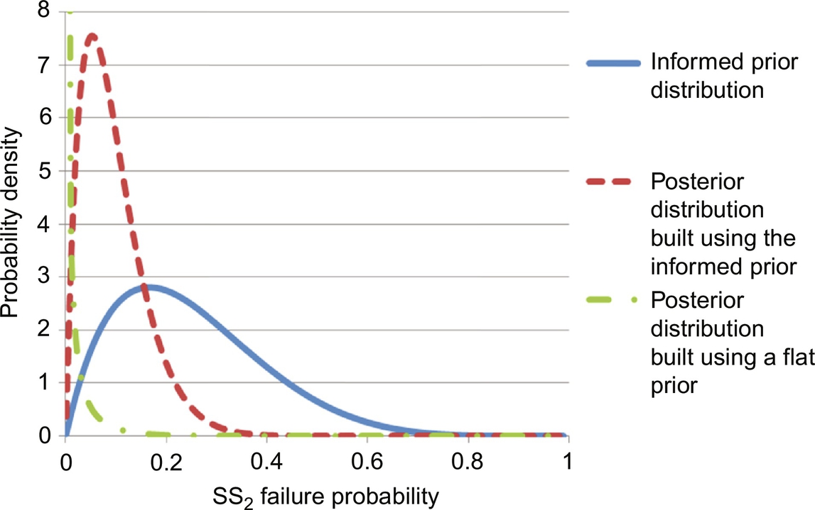
This informed prior distribution was built using dynamic simulations with first-principle models. Even with no data available to update the distribution, process engineers and plant operators can make improved risk predictions (Leveson & Stephanopolous, 2014). The alarm data are used to build a likelihood distribution, in this case a binomial likelihood distribution of a few trials, all of which are successes. Fig. 12 shows the prior and posterior distributions. The informed posterior is shifted to the left of the prior distribution by the 0% failure rate observed in the data. Unlike the commonly used uninformed prior distributions, its posterior distribution has a similar shape to its informed prior distribution. The posterior distribution generated using the informed prior distribution can alert process engineers that a significant decrease in steam pressure has the high probability (>20%) of causing a plant shutdown. This may lead operators to pay special attention to the steam pressure measurements, and may lead process engineers to install a more robust controller on the steam line.
3.4 Improvements Using Process and Response-Time Monitoring
To improve the predictions of the informed prior distribution, Moskowitz et al. (2016) proposed refinements in the models used to construct them. They began by using SS1 activations, which are infrequent, but still provide sufficient data for studying the propagation of SCEs. The activation of SS2 is rarer, occurring 1/x1 times less frequently—often resulting in very sparse data. While the data associated with SS2 are insufficient alone to analyze the performance of the safety system, the similarities between the safety systems can be utilized. The activations of both safety systems originate from a control system failure, which, for example, can be due to the large magnitude of the disturbance, the inability of the control system to handle the disturbance, and/or the occurrence of an electrical or mechanical failure. It is assumed that the same group of operators is involved. If highly skilled, they should arrest the special causes at a high rate (Chang & Mosleh, 2007; Meel et al., 2007; Meel, Seider, & Oktem, 2008).
Clearly, the need for urgent responses of SS2 is greater. Also, when operators take action (e.g., as furnace temperatures become elevated), the need to respond within the interlock delay times dominate their concerns and actions. This would normally stimulate a strong reaction to avoid automatic shutdown.
A sufficiently accurate first-principles process model is needed to implement the method of Moskowitz et al. (2016). Also, the automated safety system models should be sufficiently accurate. The second model, represented by g1(Am) in Fig. 8, is the distribution of SCE magnitudes to be simulated. The operator behavior model, g2(τ), unlike automatic safety systems, must reflect human behaviors. Here, the speed and effectiveness of operator responses often depend on the state of the process, the number of competitive active alarms, distractions, personal health and conflicts, and the like.
In the method proposed by Moskowitz et al. (2016), SS1 models are first constructed and validated with plentiful data. After constructing these models, and validating them with measured SS1 data, they are modified to handle SS2 activations (recognizing that their rare occurrences do not allow for reliable model validation). In Sections 3.4.1–3.4.3, all three models are described with respect to SS1. Their modifications to handle SS2 activations are then described. Lastly, the failure probability estimates generated by using the SS2 informed prior distributions are presented.
3.4.1 Dynamic Process Models
Because dynamic first-principles process models are widely used, approaches to model development are not considered here. Instead, this section focuses on model evaluation and improvement for constructing informed prior distributions.
Often, process engineers have developed dynamic process models for control scheme testing during the design phase. These are commonly used initially for carrying out dynamic risk analysis. However, process models used for process design and control are normally developed to track responses in their typical operating regimes (green-belt zones)—but may not respond to SCEs with sufficient accuracy; i.e., their predictions far from set points may be poor for risk analysis. Consequently, dynamic process models should often be improved to construct informed prior distributions.
For the SMR process shown in Fig. 9, four dynamic process models are constructed, as summarized in Fig. 13. The first, Process Model A, is the same as the one summarized in Section 3.2. This model includes constitutive equations to model the endothermic reformer reactions, the furnace that provides their heat, the exothermic water–gas shift reaction, the separation of hydrogen product from offgas in adsorption beds, and the production of steam (for process heating or sale), as well as models of associated PID controllers.

In Process Model A, to model the radiative heat transfer (~90% of the total heat transfer to the tubes), view factors are estimated from each surface or volume zone to each other zone, with the dynamics of radiative heat-transfer modeled between all discretized zones (Hottel & Sarofim, 1967). The remaining convective heat transfer is simpler, because heat transfer only occurs between physically adjacent zones (Lathem, McAuley, Peppley, & Raybold, 2011).
In Process Models B and D, only convection heat transfer is modeled, with radiative heat transfer accounted for by overstating the heat-transfer coefficients between the furnace gases and tube surfaces. To estimate the overstated heat-transfer coefficients, 50 steady-state windows were identified in the historical process data (Moskowitz et al., 2016). Each window corresponds to a duration of operation, on the order of a day, where process variables are at steady state. Many different steady-state windows exist in the process data due to different demand rates of hydrogen and steam, different feed ratios of steam to natural gas, and natural aging of the catalyst (in the reformer as well as the water–gas shift reactor). The heat-transfer coefficient was estimated from the temperature and flow rate of the process and furnace gas inlet and outlet measurements.
In Process Models A and B, the reforming reaction kinetics proposed by Xu and Froment (1989), which had been shown to be quite accurate over a broad range of temperatures and reactant concentrations, are used. Note that, due to the presence of a complex denominator in the kinetic equations, the spatially distributed SMR model can be difficult to converge. Accurate guess values for the concentration of the reactants and products along the axial direction of the reformer tubes must be available, or generated using homotopy-continuation techniques, to converge the steady-state model.
However, in Process Models C and D, elementary reaction kinetic equations are simpler to converge. The rate constants of the elementary reactions are estimated, similar to the convection heat-transfer coefficients. Using the data in the 50 steady-state windows, along with measured hydrogen product flow rates and offgas concentrations, the rate constants were estimated (Moskowitz et al., 2016).
Initially, the four process models were compared in the 50 steady-state windows. Beginning with the measured inlet temperatures and flow rates for each mode, predicted and measured outlet temperatures were compared for each model. The root-mean square outlet temperature differences are shown in Fig. 14. For this steady-state evaluation, Process Model A provided the best agreement with the data, whereas Process Model D was least accurate.
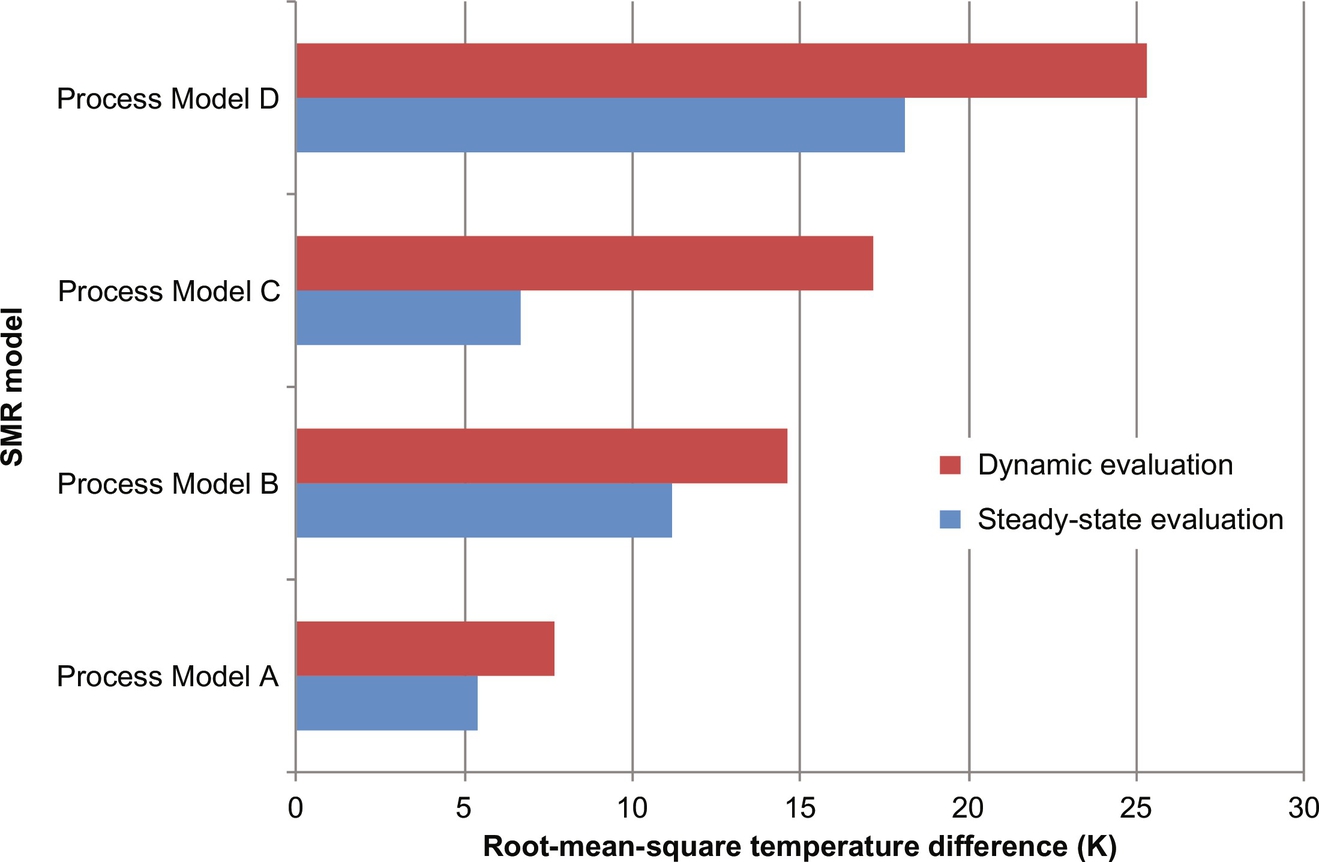
However, because the models were used to estimate the responses to SCEs, agreement with dynamics data is more important. Fifty dynamic windows were identified in the historical process data—periods of time where the process variables describing the operation of the steam-methane reforming reactor are transient. These windows are on the order of minutes to hours, and typically arise when hydrogen or steam demand rates change, feed ratios of steam to natural gas change, or operational changes occur in another process unit (such as a pair of pressure-swing adsorbent beds are taken offline). For each of the 50 dynamic windows, inlet temperature and flow rate trajectories were input to each model, with model-predicted outlet temperature trajectories compared to measured outlet temperature trajectories. Dynamic predictions are typically less accurate than the steady-state ones. Here, Process Model B outperformed Process Model C, but when comparing just steady-state outlet temperature differences, Process Model C provided a closer fit to the data. Clearly, Process Model B should be selected, rather than Process Model C, when constructing informed prior distributions.
Next, the four process models were used to construct informed prior distributions for the failure of SS1—using the uniform distributions for special-cause magnitude and operator behavior used in Section 3.3. The 300 measured SS1 failures/successes were then used to construct a low-variance binomial likelihood distribution (see Eq. 4 in Moskowitz et al., 2016). The four informed prior distributions for the failure of SS1 and the binomial distribution are shown in Fig. 15. To compare the four informed prior distributions with this likelihood distribution, the index
was used, where i represents the model (i=A, B, C, D) and m represents the data-based likelihood distribution. This index ranges from [0, 1], where unity corresponds to perfect matching between the informed prior distribution of model i and the measured likelihood distribution m. As shown in Table 3, this index is consistent with the dynamic model accuracies in Fig. 14, but low levels of agreement are obtained. Note that using more detailed operator response-time models, in the next subsection, the performance indices are improved significantly.

3.4.2 SCE Occurrence Model
When constructing informed prior distributions to estimate the failure probabilities of safety systems that act infrequently, it is important to assess the SCEs that can activate specific safety systems. Given that process units fail in many ways (e.g., as inlet stream compositions, temperatures, flow rates, and pressures vary; controllers experience measurement bias; valves malfunction; controller electronic mechanisms fail), special-cause modeling deserves attention. Clearly, for specific SCEs, known to trigger safety systems, it is crucial to account for them when creating informed prior distributions. Some are known to have a high likelihood of occurrence over the lifetime of a plant, while others may be unobserved locally, having occurred at other plant sites or even related plants. For all potential SCEs, a probability distribution should be constructed, even when likelihood data are unavailable.
When developing occurrence models to estimate safety system failure probabilities, SCEs must be selected and their magnitudes must be investigated, as SCEs are likely to have devastating consequences (e.g., propagation of runaway reactions, leading to explosions). To identify these events, HAZOP and LOPA analyses, especially, are particularly helpful. HAZOP is the industry standard for postulating all possible SCEs.
The effect of an SCE depends on its magnitude. SCE models (e.g., g1(Am) in Fig. 8) are needed to estimate failure probability distributions. SCE models having low expected values are most representative and rarely activate second-level alarms, while SCE models having high expected values represent extreme cases, allowing for the study of second-level alarms. Various steam pressure decrease magnitudes are shown in Fig. 16—each being a delta function centered at its corresponding point on the abscissa. The expected value of the SS1 failure probability, jm, is graphed accordingly.
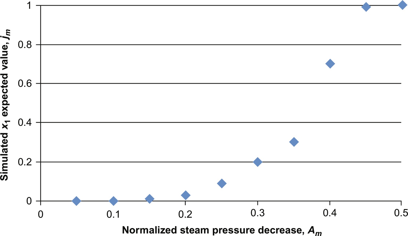
3.4.3 Operator Response-Time Models
In the simulation of a SCE, Moskowitz et al. (2016) show that the behavior of the operator must be well understood. In Fig. 8, g2(τ) represents operator response times in taking action following activated alarms associated with SS1. An initial construction of g2(τ) can be made using the histogram of operator response times to high-frequency alarms. This provides valuable information about how the operators tend to act when a variable is under alarm (Bendoly, Donohue, & Schultz, 2006; Macwan & Mosleh, 1994; Stylios & Groumpos, 1999). In some cases, when operators anticipate that the alarm thresholds have been set conservatively, they are slower to respond to expected nuisance alarms. On the other hand, when operators recognize that alarms tend to trigger a flood of alarms elsewhere in the process, they view these alarms as critical—even though they just signal entry into the yellow-belt zone. To the extent possible, it is important to make quantifiable justifications when modeling operator effectiveness (Hollnagel, 1998; Reason, 2000).
A histogram of approximately 300 observed operator response times to the H-alarm associated with the SMR furnace effluent temperature (Moskowitz et al., 2016) is shown in Fig. 17. The operator response times were collected using the alarm data log, which recorded the time of each alarm activation and the time of each operator manipulation. The time between an alarm activation and the initial operator manipulation is the operator response time. This calculation method provides the most accurate data on operator response time. Alarm data are convenient to work with, but without alarm data, process data can be sampled to obtain operator response times. A script can be written to record the times process variables cross their thresholds, as well as the times controlled-variable set points or actuators undergo step changes (considered to be operator actions) (Pariyani et al., 2012a). In either case, the data sampling interval is important to consider. If data are sampled or recorded infrequently (such as by a composition analyzer), operator response times may be inaccurate. Depending upon the frequency of process data points, reasonable estimates of operator response times can be obtained. The wide range of operator response times, nearly all well represented, suggest many kinds of operator actions. The highest number of responses is associated with the shortest response times—with operators taking action in less than 1 min. Nearly all of the operator response times lie between 0 and 6 min, with far fewer of longer duration. Past a 6 min response time, the number of responses decreases rapidly, with just three response times beyond 8 min.
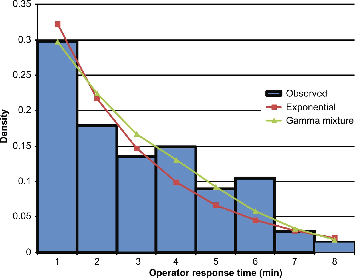
Two parametric distributions were used to model the operator response-time distribution. The first distribution is an exponential distribution, which is called Operator Response-Time Model A:
where λ is a parameter to be estimated by maximizing the likelihood function:

where i is the response counter, n is the total number of response times measured (on the order of 300), and τi is response-time i. It is often convenient to maximize the log-likelihood function instead of the likelihood function:
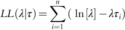
The maximum of the log-likelihood function has a simple analytical form:
where  is the sample mean of the measured response times.
The second is a weighted sum of three gamma distributions (Operator Response-Time Model B):
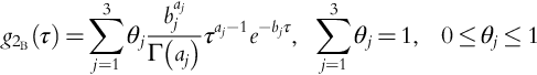
where each θj is a weighting coefficient for gamma distribution j, and where aj and bj are the parameters of gamma distribution j. While any number of gamma distributions can be used, here the fourth distribution gives a negligible increase in the likelihood function (compared to the impact of the third distribution). The eight parameters in Eq. (16) are estimated by maximizing the likelihood function:
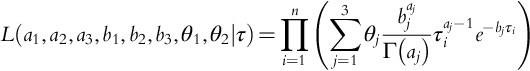
Using Newton's optimization method with an analytical Hessian matrix, the parameter values in Table 4 were estimated.
Table 4
Parameters for Operator Response-Time Models A and B
| λ | a1 | a2 | a3 | b1 | b2 | b3 | θ1 | θ2 | θ3 |
| 0.39 | 1.83 | 3.56 | 4.51 | 0.68 | 1.04 | 0.88 | 0.48 | 0.07 | 0.45 |
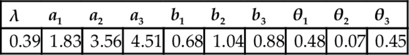
While Operator Response-Time Models A and B represent operator response times well, they do not account for the rate of change of each variable crossing its alarm threshold, as well as the number of activated alarms being monitored by an operator(s). Clearly, operator responses gain urgency, and often speed, when a variable crosses one of its thresholds rapidly. Also, as the number of active alarms decreases, operators are less distracted and respond more rapidly.
To account for the rate of change of each variable when the variable crosses an alarm threshold, using the SMR plant data, operator response times are displayed in Fig. 18 as a function of the furnace effluent temperature derivative, dx/dt, as the temperature crosses its high-alarm threshold (Moskowitz et al., 2016). The dependence of the operator response time, τ, on the rate of change is well described by:
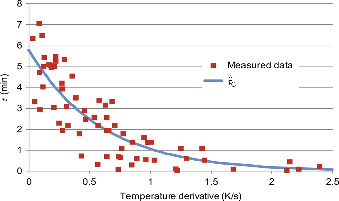
where κ1 and ν1 are the model parameters. These parameters are estimated by minimizing the sum of the squared errors:
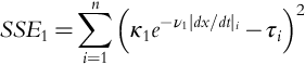
The estimated values of κ1 and ν1 as well as the corresponding SSE1 value are given in Table 5.
Table 5
Parameters Used for Operator Response-Time Models C–E
| κ1 (min) | ν1 (s/K) | SSE1 | κ2 (min) | ν2 (1/no. of alarms) | SSE2 |
| 4.33 | 1.54 | 302 | 3.8 | 4.2 | 413 |
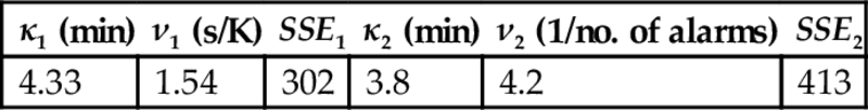
To construct a g2(τ) that accounts for the alarmed variable time derivative, a stochastic component must be maintained—because if g2(τ) were purely deterministic (like ![]() ), the variance of the safety system failure probability with respect to Am cannot be calculated. While
), the variance of the safety system failure probability with respect to Am cannot be calculated. While ![]() is an estimate for the operator response time, it must be incorporated into a random variable distribution for τ. One choice for g2(τ) is the exponential distribution having an expected value equal to
is an estimate for the operator response time, it must be incorporated into a random variable distribution for τ. One choice for g2(τ) is the exponential distribution having an expected value equal to ![]() . The exponential distribution in Eq. (17) is known to have an expected value of 1/λ. Therefore, Operator Response-Time Model C is proposed:
. The exponential distribution in Eq. (17) is known to have an expected value of 1/λ. Therefore, Operator Response-Time Model C is proposed:

A similar method can be used to account for the effect of multiple alarm activations in the process. When many alarms are active, competing for operator(s) attention, response times are expected to increase. Here, also, the exponential distribution is appropriate:
where γ is the reciprocal of active alarms. The parameters κ2 and ν2 are estimated by minimizing the sum of the squared errors:
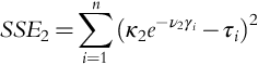
The estimated values for κ2 and ν2 as well as the corresponding SSE2 value are given in Table 6.
Table 6
Performance Index for Operator Response-Time Models A–E With Process Model A
| ORTM A | ORTM B | ORTM C | ORTM D | ORTM E | |
| ξi,m | 0.029 | 0.030 | 0.633 | 0.701 | 0.812 |
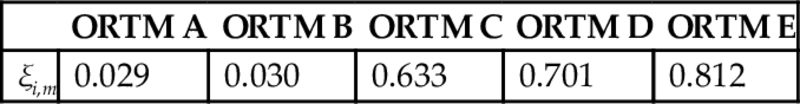
Using this logic, the Operator Response-Time Model D is formulated by setting the expected value of an exponential distribution equal to ![]() :
:
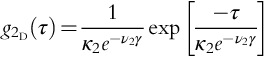
Finally, the Operator Response-Time Model E is formulated that incorporates both ![]() and
and ![]() . The effectiveness of
. The effectiveness of ![]() and
and ![]() can be compared by their associated SSEs. In Moskowitz et al. (2016), the expected value of Operator Response Model E is set equal to:
can be compared by their associated SSEs. In Moskowitz et al. (2016), the expected value of Operator Response Model E is set equal to:
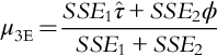
where the weighting coefficients for each distribution are proportional to their SSEs. This yields Operator Response-Time E model:
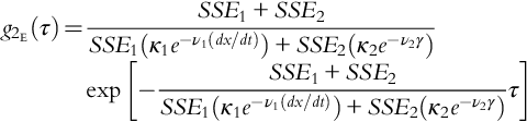
Next, Operator Response-Time Models A–E are used to construct informed prior distributions for the failure probability of SS1, along with dynamic Process Model A. The results are shown in Fig. 19, along with the binomial likelihood distribution of the measured SS1 data, Eq. (4). The model performance index, ξi,m, in Eqs. (3a) and (3b) is used to quantify the model performance of Operator Response-Time Models A–E, with results shown in Table 6. Operator Response-Time Models A and B, which are independent of the process state, describe the measured alarm data poorly. As expected, Operator Response-Time Model B, with eight parameters, performs better than Operator Response-Time Model A, with just a single parameter. The incorporation of ![]() and
and ![]() in Operator Response-Time Models C and D, clearly improves the informed prior distributions, with Model C performing better than Model D—expected because
in Operator Response-Time Models C and D, clearly improves the informed prior distributions, with Model C performing better than Model D—expected because ![]() Of the five models, Model E is in the closest agreement with the likelihood data. Given preferred Model E, the choice of process model can be revisited. In Fig. 20, the four dynamic process models are used to build informed prior distributions with Operator Response-Time Model E. The model performance indices are shown for Process Models A–D in Table 7. Once again, Process Model A yields the best agreement with the observed likelihood data and can be considered the most appropriate process model.
Of the five models, Model E is in the closest agreement with the likelihood data. Given preferred Model E, the choice of process model can be revisited. In Fig. 20, the four dynamic process models are used to build informed prior distributions with Operator Response-Time Model E. The model performance indices are shown for Process Models A–D in Table 7. Once again, Process Model A yields the best agreement with the observed likelihood data and can be considered the most appropriate process model.
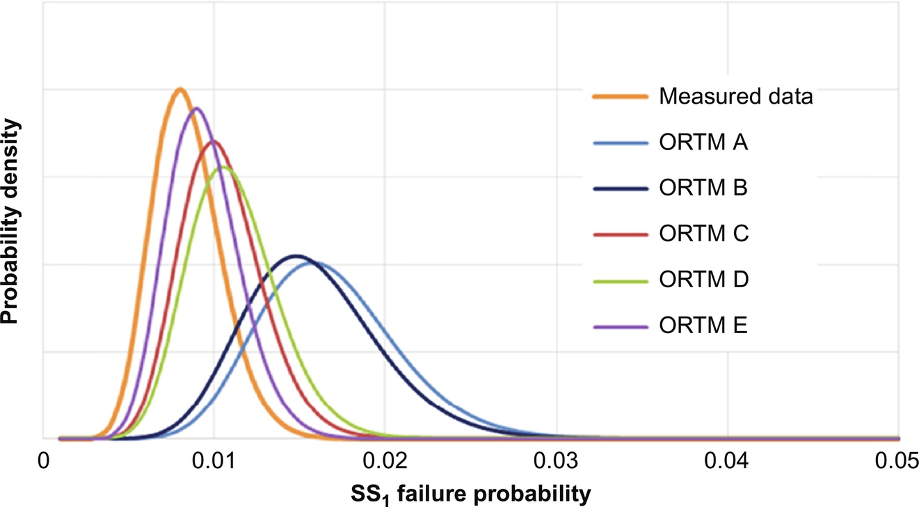
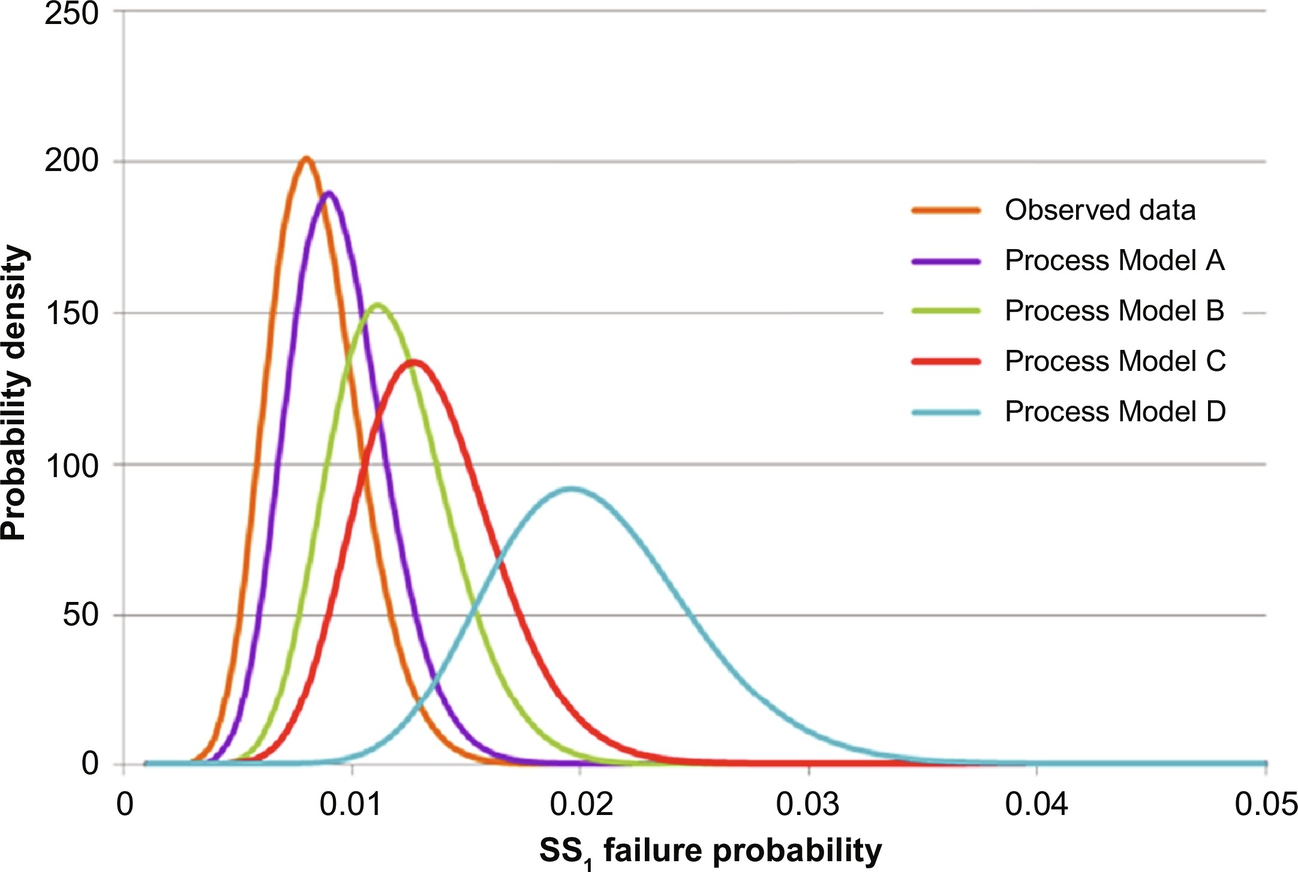

3.5 Modeling SS2 Failures Using Models With Parameters Estimated From SS1 Failures
Once the three types of models (process, SCE, and operator response-time models) are chosen and their parameters are estimated, Moskowitz et al. (2016) use them to estimate the failure probabilities of SS1. These models must then be adjusted to handle simulations that involve the activation of SS2 (i.e., after the failure of SS1). While it is desirable to keep the models intact, a few adjustments are recommended (Moskowitz et al., 2016).
The dynamic process model, Process Model A, should not be altered much to simulate SS2 activation events for the SMR—because the simulations from high and high–high alarms, and beyond, are similar, with small changes in physical properties as temperatures rise. In general, Process Model A adjustments would be required when physical and chemical phenomena change abruptly—for example, with shifts from laminar to turbulent flows, or the introduction of two-phase flows.
The SCE Occurrence Model needs significant adjustment because the g1(Am) distribution used for simulating L/H alarm activations infrequently activates LL/HH alarms. To achieve this, a normal distribution is chosen for g1(Am), having mean ![]() and standard deviation σ. A lower-tail, bounded by θL and an upper-tail bounded by θU, each two standard deviations from the mean, are defined:
and standard deviation σ. A lower-tail, bounded by θL and an upper-tail bounded by θU, each two standard deviations from the mean, are defined:
noting that θL is a special-cause magnitude closer to zero; that is, closer to typical operation. The normal distribution is described by θL and θU, rather than the typical mean and standard deviation:

The lower bound of θL is set at Am values for which the L/H alarms failed in simulation—with smaller choices of θL yielding many simulations where the LL/HH alarms are not activated. Referring to Fig. 16, with SS1 failures frequently observed when ![]() , 0.4 is a good lower bound for θL. θU is set such that the SCEs are of interest and relevance. Three SCE occurrence models are shown in Fig. 21, each sharing
, 0.4 is a good lower bound for θL. θU is set such that the SCEs are of interest and relevance. Three SCE occurrence models are shown in Fig. 21, each sharing ![]() . SCEM A has θU closest to θL, and samples SCEs that are most likely (closest to typical operation), yet have the least potential for SS2 failures. The other extreme is SCEM C, which has θU furthest from θL.. SCEM B, having
. SCEM A has θU closest to θL, and samples SCEs that are most likely (closest to typical operation), yet have the least potential for SS2 failures. The other extreme is SCEM C, which has θU furthest from θL.. SCEM B, having ![]() is chosen as an interior candidate to analyze the risk of SS2 failures. The choice of g1(Am) has a significant impact on the estimated failure probabilities—the user must keep this in mind when analyzing the simulation results and making statements about the risk of the process. The failure probability estimate attempts to describe the probability of failure while undergoing a SCE sampled from g1(Am), which is very different than typical day-to-day process fluctuations.
is chosen as an interior candidate to analyze the risk of SS2 failures. The choice of g1(Am) has a significant impact on the estimated failure probabilities—the user must keep this in mind when analyzing the simulation results and making statements about the risk of the process. The failure probability estimate attempts to describe the probability of failure while undergoing a SCE sampled from g1(Am), which is very different than typical day-to-day process fluctuations.
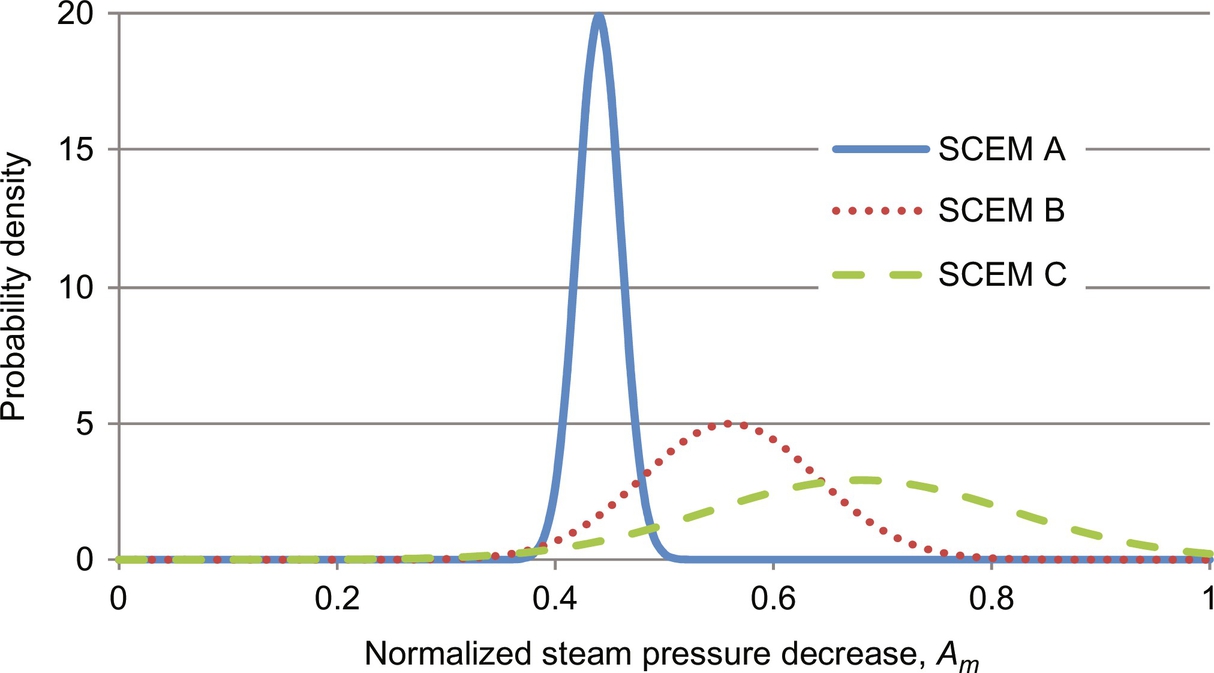
The Operator Response-Time Models also need adjustment, it being expected that operators react quicker to alarm activations that are associated with more urgent consequences. Given an immediate threat of an automatic plant shutdown, operator actions should be accelerated. To account for this, when SS1 is activated to SS2, the time response to the SS2 activation is divided by the ratio of the 90% percentile of operator response to a SS1 activation, τ90%, over the interlock shutdown time, Δtint. For this case, the Operator Response-Time Model E takes the form:
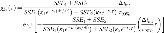
Having constructed, chosen, and regressed the three types of models using the H-alarm data, Moskowitz et al. (2016) make adjustments to model SS2 activation events. An informed prior distribution is then constructed for the failure probabilities of SS2. Fig. 22 shows the resulting informed prior and associated posterior distributions describing the failure probability of SS2. The sparse alarm data are used to build binomial likelihood distributions that modify the prior distributions to form posterior distributions. It can be seen that the most accurate posterior distribution (formed using Process Models A and Operator Response-Time Model E with an urgency adjustment for time responses in SS2) is not shifted as dramatically as the posterior distribution formed using the simple informed prior distribution. This indicates that the most accurate posterior distribution is more effective at handling the special-cause simulations—leading to more accurate failure probability predictions.
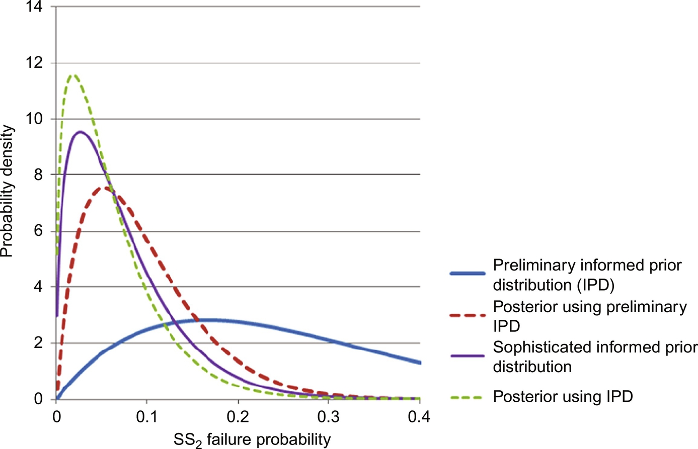
The interpretation of the posterior distribution is that during a severe loss in steam pressure, the probability that the process will undergo an automatic shutdown is on the order of 5%. This allows engineers responsible for setting reliability estimates to have quantifiable justification when they do so. An estimate for the reliability for various SCEs can provide engineers with a broader understanding of the events that pose the greatest odds of an interlock activation, thus motivating different designs to handle these events. The operator also benefits from these distributions, as he/she becomes aware that, during such severe pressure drops, his/her reactions have been projected to result in interlock activations after on the order of 5% of occurrences. If this value is perceived to be too high, the operator may be motivated to act more urgently during this type of event.
4 Summary
The rapid development of dynamic risk analyses, over the past 2 decades, has been reviewed, principally to introduce many techniques to chemical process safety practitioners/researchers. Initial strategies involved Bayesian analysis with copulas to model the failure probabilities of safety systems when responding to rare alarms. For safety interlock systems and their associated alarms, statistical techniques on the sparse records of activations are alone insufficient to make meaningful evaluations of their failure probabilities. With process models, the use of operator response data associated with the relatively frequent alarm activations (e.g., H alarms), that is, plentiful near miss operator data, are examined. Better estimates were obtained using improved process/operator models to inform prior failure probability distributions. The latter are very promising for improving the failure probability estimates of safety systems associated with less frequently activated alarms (e.g., HH alarms) and safety interlock systems; that is, to provide more reliable safety risk analyses.