Search in book...
Toggle Font Controls
Create new playlist

Name your new playlist

Playlist description (optional)
Sign In

Email address

Password

Forgot Password?

or

Continue with Facebook

Continue with Google
Sign Up

Full Name

Email address

Confirm Email Address

Password

or

Continue with Facebook

Continue with Google

Chapter 10

Image Dehazing: Improved Techniques

Yu Liu^⁎; Guanlong Zhao^†; Boyuan Gong^†; Yang Li^⁎; Ritu Raj^†; Niraj Goel^†; Satya Kesav^†; Sandeep Gottimukkala^†; Zhangyang Wang^†; Wenqi Ren^‡; Dacheng Tao^§ ^⁎Department of Electrical and Computer Engineering, Texas A&M University, College Station, TX, United States
^†Department of Computer Science and Engineering, Texas A&M University, College Station, TX, United States
^‡Chinese Academy of Sciences, Beijing, China
^§University of Sydney, Sydney, NSW, Australia

Abstract

Image dehazing has been recently studied intensively in the fields of computational photography and computer vision, using deep learning approaches. Here we explore two related but important tasks based on the recently released REalistic Single Image DEhazing (RESIDE) benchmark dataset: (i) single image dehazing as a low-level image restoration problem; and (ii) high-level visual understanding (e.g., object detection) of hazy images. For the first task, we investigated a variety of loss functions and show that perception-driven loss significantly improves dehazing performance. In the second task, we provide multiple solutions including using advanced modules in the dehazing–detection cascade and domain-adaptive object detectors. In both tasks, our proposed solutions significantly improve performance. GitHub repository URL: https://github.com/guanlongzhao/dehaze.

Keywords

Image dehazing; Restoration and enhancement; Domain adaptation; Deep learning

10.1 Introduction

In many emerging applications such as autonomous/assisted driving, intelligent video surveillance, and rescue robots, the performances of visual sensing and analytics are largely jeopardized by various adverse visual conditions, e.g., bad weather and illumination conditions from the unconstrained and dynamic environments. While most current vision systems are designed to perform in clear environments, i.e., where subjects are well observable without (significant) attenuation or alteration, a dependable vision system must reckon with the entire spectrum of complex unconstrained outdoor environments. Taking autonomous driving, for example, the industry players have been tackling the challenges posed by inclement weather; however, heavy rain, haze or snow will still obscure the vision of on-board cameras and create confusing reflections and glare, leaving the state-of-the-art self-driving cars in a struggle. Another illustrative example can be found in video surveillance cameras: even the commercialized cameras adopted by governments appear fragile in challenging weather conditions. Therefore, it is highly desirable to study to what extent, and in what sense, such adverse visual conditions can be coped with, for the goal of achieving robust computer vision systems in the wild that benefit security/safety, autonomous driving, robotics, and an even broader range of applications.

Despite the blooming research on relevant topics, such as dehazing and rain removal, a unified view towards these problems has been absent, so have collective efforts for resolving their common bottlenecks. On the one hand, such adverse visual conditions usually give rise to complicated, nonlinear and data-dependent degradations, which follow some parameterized physical models a priori. This will naturally motivate a combination of model-based and data-driven approaches. On the other hand, most existing research works confined themselves to solving image restoration or enhancement problems. In contrast, general image restoration and enhancement, known as part of low-level vision tasks, are usually thought as the preprocessing step for mid- and high-level vision tasks. The performance of high-level computer vision tasks, such as object detection, recognition, segmentation and tracking, will deteriorate in the presence of adverse visual conditions, and is largely affected by the quality of handling those degradations. It is thus highly meaningful to examine whether restoration-based approaches for alleviating adverse visual conditions would actually boost the target high-level task performance or not. Lately, there have been a number of works exploring the joint consideration of low- and high-level vision tasks as a pipeline and achieving superior performance.

This chapter takes image dehazing as a concrete example to illustrate the handling of the above challenges. Images taken in outdoor environments affected by air pollution, dust, mist, and fumes often contain complicated, nonlinear, and data-dependent noise, also known as haze. Haze complicates many high-level computer vision tasks such as object detection and recognition. Therefore, dehazing has been widely studied in the fields of computational photography and computer vision. Early dehazing approaches often required additional information such as the provision or capture of scene depth by comparing several different images of the same scene [1–3]. Many approaches have since been proposed to exploit natural image priors and to perform statistical analyses [4–7]. Most recently, dehazing algorithms based on neural networks [8–10] have delivered state-of-the-art performance. For example, AOD-Net [10] trains an end-to-end system and shows superior performance according to multiple evaluation metrics, improving object detection in the haze using end-to-end training of dehazing and detection modules.

10.2 Review and Task Description

Here we study two haze-related tasks: (i) boosting single image dehazing performance as an image restoration problem; and (ii) improving object detection accuracy in the presence of haze. As noted by [11,10,12], the second task is related to, but is often unaligned with, the first.

While the first task has been well studied in recent works, we propose that the second task is more relevant in practice and deserves greater attention. Haze does not affect human visual perceptual quality as much as resolution, noise, and blur; indeed, some hazy photos may even have better aesthetics. However, haze in unconstrained outdoor environments could be detrimental to machine vision systems, since most of them only work well for haze-free scenes. Taking autonomous driving as an example, hazy and foggy weather will obscure the vision of on-board cameras and create confusing reflections and glare, creating problems even for state-of-the-art self-driving cars [12].

10.2.1 Haze Modeling and Dehazing Approaches

An atmospheric scattering model has been widely used to represent hazy images in haze removal works [13–15]:

$I (x) = J (x) t (x) + A (1 - t (x)),$ $I (x) = J (x) t (x) + A (1 - t (x)),$

(10.1)

where x indexes pixels in the observed hazy image, $I (x)$ $I (x)$ is the observed hazy image, and $J (x)$ $J (x)$ is the clean image to be recovered. Parameter A denotes the global atmospheric light, and $t (x)$ $t (x)$ is the transmission matrix defined as

$t (x) = e^{- β d (x)},$ $t (x) = e^{- β d (x)},$

(10.2)

where β is the scattering coefficient, and $d (x)$ $d (x)$ represents the distance between the object and camera.

Conventional single image dehazing methods commonly exploit natural image priors (for example, the dark channel prior (DCP) [4,5], the color attenuation prior [6], and the non-local color cluster prior [7]) and perform statistical analysis to recover the transmission matrix $t (x)$ $t (x)$ . More recently, convolutional neural networks (CNNs) have been applied for haze removal after demonstrating success in many other computer vision tasks. Some of the most effective models include the multi-scale CNN (MSCNN) which predicts a coarse-scale holistic transmission map of the entire image and refines it locally [9]; DehazeNet, a trainable transmission matrix estimator that recovers the clean image combined with estimated global atmospheric light [8]; and the end-to-end dehazing network, AOD-Net [10,16], which takes a hazy image as input and directly generates a clean image output. AOD-Net has also been extended to video [17].

10.2.2 RESIDE Dataset

We benchmark against the REalistic Single Image DEhazing (RESIDE) dataset [12]. RESIDE was the first large-scale dataset for benchmarking single image dehazing algorithms and includes both indoor and outdoor hazy images.¹ Further, RESIDE contains both synthetic and real-world hazy images, thereby highlighting diverse data sources and image contents. It is divided into five subsets, each serving different training or evaluation purposes. RESIDE contains $110, 500$ $110, 500$ synthetic indoor hazy images (ITS) and $313, 950$ $313, 950$ synthetic outdoor hazy images (OTS) in the training set, with an option to split them for validation. The RESIDE test set is uniquely composed of the synthetic objective testing set (SOTS), the annotated real-world task-driven testing set (RTTS), and the hybrid subjective testing set (HSTS) containing 1000, 4332, and 20 hazy images, respectively. The three test sets address different evaluation viewpoints including restoration quality (PSNR, SSIM and no-reference metrics), subjective quality (rated by humans), and task-driven utility (using object detection, for example).

Most notably, RTTS is the only existing public dataset that can be used to evaluate object detection in hazy images, representing mostly real-world traffic and driving scenarios. Each image is annotated with object bounding boxes and categories (person, bicycle, bus, car, or motorbike). Furthermore, 4807 unannotated real-world hazy images are also included in the dataset for potential domain adaptation.

For Task 1, we used the training and validation sets from ITS + OTS, and the evaluation is based on PSNR and SSIM. For Task 2, we used the RTTS set for testing and evaluated using mean average precision (MAP) scores.

10.3 Task 1: Dehazing as Restoration

Most CNN dehazing models [8–10] refer to the mean-squared error (MSE) or $ℓ_{2}$ $ℓ_{2}$ norm-based loss functions. However, MSE is well-known to be imperfectly correlated with human perception of image quality [18,19]. Specifically, for dehazing, the $ℓ_{2}$ $ℓ_{2}$ norm implicitly assumes that the degradation is additive white Gaussian noise, which is oversimplified and invalid for haze. On the other hand, the $ℓ_{2}$ $ℓ_{2}$ norm treats the impact of noise independently of the local image characteristics such as structural information, luminance and contrast. However, according to [20], the sensitivity of the Human Visual System (HVS) to noise depends on the local properties and structure of a vision.

Here we aimed to identify loss functions that better match human perception to train a dehazing neural network. We used AOD-Net [10] (originally optimized using MSE loss) as the backbone but replaced its loss function with the following options:

• $ℓ_{1}$ $ℓ_{1}$ loss. The $ℓ_{1}$ $ℓ_{1}$ loss for a patch P can be written as:

$L^{ℓ_{1}} (P) = \frac{1}{N} \sum_{p \in P} | x (p) - y (p) |,$ $L^{ℓ_{1}} (P) = \frac{1}{N} \sum_{p \in P} | x (p) - y (p) |,$

(10.3)

where N is the number of pixels in the patch, p is the index of the pixel, and $x (p)$ $x (p)$ and $y (p)$ $y (p)$ are the pixel values of the generated and the ground-truth images, respectively.
• SSIM loss. Following [19], we write the SSIM for pixel p as:

$\begin{matrix} S S I M (p) & = \frac{2 μ_{x} μ_{y} + C_{1}}{μ_{x}^{2} + μ_{y}^{2} + C_{1}} \cdot \frac{2 σ_{x y} + C_{2}}{σ_{x}^{2} + σ_{y}^{2} + C_{2}} \\ = l (p) \cdot c s (p) . \end{matrix}$ $\begin{matrix} S S I M (p) & = \frac{2 μ_{x} μ_{y} + C_{1}}{μ_{x}^{2} + μ_{y}^{2} + C_{1}} \cdot \frac{2 σ_{x y} + C_{2}}{σ_{x}^{2} + σ_{y}^{2} + C_{2}} \\ = l (p) \cdot c s (p) . \end{matrix}$

(10.4)

The means and standard deviations are computed using a Gaussian filter with standard deviation $σ_{G}$ $σ_{G}$ . The loss function for SSIM can then be defined as

$L^{S S I M} (P) = \frac{1}{N} \sum_{p \in P} 1 - S S I M (p) .$ $L^{S S I M} (P) = \frac{1}{N} \sum_{p \in P} 1 - S S I M (p) .$

(10.5)

• MS-SSIM loss. The choice of $σ_{G}$ $σ_{G}$ would impact the training performance of SSIM. Here we adopt the idea of multi-scale SSIM [19], where M different values of $σ_{G}$ $σ_{G}$ are pre-chosen and fused:

$L^{M S - S S I M} (P) = l_{M}^{α} (p) \cdot \prod_{j = 1}^{M} c s_{j}^{β_{j}} (P) .$ $L^{M S - S S I M} (P) = l_{M}^{α} (p) \cdot \prod_{j = 1}^{M} c s_{j}^{β_{j}} (P) .$

(10.6)

• MS-SSIM+ $ℓ_{2}$ $ℓ_{2}$ loss. Using a weighted sum of MS-SSIM and $ℓ_{2}$ $ℓ_{2}$ as the loss function,

$L^{M S - S S I M - ℓ_{2}} = α \cdot L^{M S S S I M} + (1 - α) \cdot G_{σ_{G}^{M}} \cdot L^{ℓ_{2}},$ $L^{M S - S S I M - ℓ_{2}} = α \cdot L^{M S S S I M} + (1 - α) \cdot G_{σ_{G}^{M}} \cdot L^{ℓ_{2}},$

(10.7)

a point-wise product between $G_{σ_{G}^{M}}$ $G_{σ_{G}^{M}}$ and $L^{ℓ_{2}}$ $L^{ℓ_{2}}$ is added to the $ℓ_{2}$ $ℓ_{2}$ loss function term, because MS-SSIM propagates the error at pixel q based on its contribution to MS-SSIM of the central pixel $\tilde{q}$ $\tilde{q}$ , as determined by the Gaussian weights.
• MS-SSIM+ $ℓ_{1}$ $ℓ_{1}$ loss. Using a weighted sum of MS-SSIM and $ℓ_{1}$ $ℓ_{1}$ as the loss function,

$L^{M S S S I M - ℓ_{1}} = α \cdot L^{M S S S I M} + (1 - α) \cdot G_{σ_{G}^{M}} \cdot L^{ℓ_{1}},$ $L^{M S S S I M - ℓ_{1}} = α \cdot L^{M S S S I M} + (1 - α) \cdot G_{σ_{G}^{M}} \cdot L^{ℓ_{1}},$

(10.8)

the $ℓ_{1}$ $ℓ_{1}$ loss is similarly weighted by $G_{σ_{G}^{M}}$ $G_{σ_{G}^{M}}$ .

We selected 1000 images from ITS + OTS as the validation set and the remaining images for training. The initial learning rate and mini-batch size of the systems were set to 0.01 and 8, respectively, for all methods. All weights were initialized as Gaussian random variables, unless otherwise specified. We used a momentum of 0.9 and a weight decay of 0.0001. We also clipped the $ℓ_{2}$ $ℓ_{2}$ norm of the gradient to be within $[- 0.1, 0.1]$ $[- 0.1, 0.1]$ to stabilize network training. All models were trained on an Nvidia GTX 1070 GPU for around 14 epochs, which empirically led to convergence. For SSIM loss, $σ_{G}$ $σ_{G}$ was set to 5; $C_{1}$ $C_{1}$ and $C_{2}$ $C_{2}$ in (10.4) were 0.01 and 0.03, respectively. For MS-SSIM losses, multiple Gaussian filters were constructed by setting $σ_{G}^{i} = {0.5, 1, 2, 4, 8}$ $σ_{G}^{i} = {0.5, 1, 2, 4, 8}$ ; α was set as 0.025 for MS-SSIM+ $ℓ_{1}$ $ℓ_{1}$ , and 0.1 for MS-SSIM+ $ℓ_{2}$ $ℓ_{2}$ , following [19].

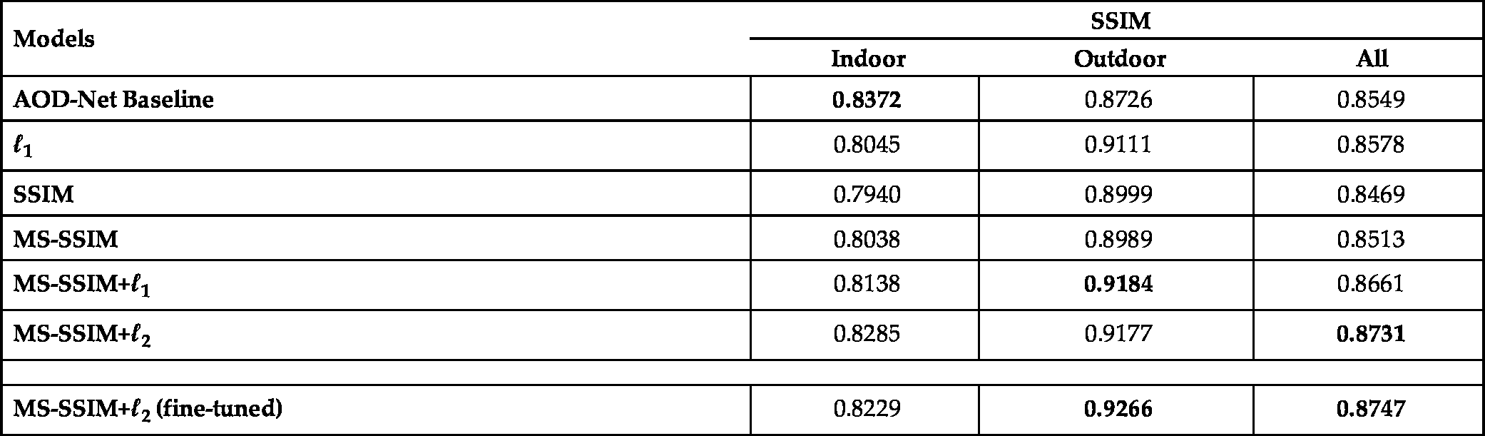
As shown in Tables 10.1 and 10.2, simply replacing the loss functions resulted in noticeable differences in performance. While the original AOD-Net with MSE loss performed well on indoor images, it was less effective on outdoor images, which are usually the images needing to be dehazed in practice. Of all the options, MS-SSIM- $ℓ_{2}$ $ℓ_{2}$ achieved both the highest overall PSNR and SSIM results, resulting in 0.88 dB PSNR and 0.182 SSIM improvements over the state-of-the-art AOD-Net. We further fine-tuned the MS-SSIM- $ℓ_{2}$ $ℓ_{2}$ model, including using a pre-trained AOD-Net as a warm initialization, adopting a smaller learning rate (0.002) and a larger minibatch size (16). Finally, the best achievable PSNR and SSIM were 23.43 dB and 0.8747, respectively. Note that the best SSIM represented a nearly 0.02 improvement over AOD-Net.

Table 10.1

Comparison of PSNR results (dB) for Task 1

Models	PSNR
Models	Indoor	Outdoor	All
AOD-Net Baseline	21.01	24.08	22.55
ℓ ₁	20.27	25.83	23.05
SSIM	19.64	26.65	23.15
MS-SSIM	19.54	26.87	23.20
MS-SSIM+ℓ₁	20.16	26.20	23.18
MS-SSIM+ℓ₂	20.45	26.38	23.41

MS-SSIM+ℓ₂ (fine-tuned)	20.68	26.18	23.43

Table 10.2

Comparison of SSIM results for Task 1

Models	SSIM
Models	Indoor	Outdoor	All
AOD-Net Baseline	0.8372	0.8726	0.8549
ℓ ₁	0.8045	0.9111	0.8578
SSIM	0.7940	0.8999	0.8469
MS-SSIM	0.8038	0.8989	0.8513
MS-SSIM+ℓ₁	0.8138	0.9184	0.8661
MS-SSIM+ℓ₂	0.8285	0.9177	0.8731

MS-SSIM+ℓ₂ (fine-tuned)	0.8229	0.9266	0.8747

10.4 Task 2: Dehazing for Detection

10.4.1 Solution Set 1: Enhancing Dehazing and/or Detection Modules in the Cascade

In [10], the authors proposed a cascade of AOD-Net dehazing and Faster-RCNN [21] detection modules to detect objects in hazy images. We therefore considered it intuitive to try different combinations of more powerful dehazing/detection modules in the cascade. Note that such a cascade could be subject to further joint optimization, as many previous works [22,23,10]. However, to be consistent with the results in [12], all detection models used in this section were the original pre-trained versions, without any retraining or adaptation.

Our solution set 1 considered several popular dehazing modules including DCP [4], DehazeNet [8], AOD-Net [10], and the recently proposed densely connected pyramid dehazing network (DCPDN) [24]. Since hazy images tend to have lower contrast, we also included a contrast enhancement method called contrast limited adaptive histogram equalization (CLAHE). Regarding the choice of detection modules, we included Faster R-CNN [21],² SSD [26], RetinaNet [27], and Mask-RCNN [28].

The compared pipelines are shown in Table 10.3. In each pipeline, “X+Y” by default means applying Y directly on the output of X in a sequential manner. The most important observation is that simply applying more sophisticated detection modules is unlikely to boost the performance of the dehazing–detection cascade, due to the domain gap between hazy/dehazed and clean images (on which typical detectors are trained). The more sophisticated pre-trained detectors (RetinaNet, Mask-RCNN) may have overfitted the clean image domain, again highlighting the demand of handling domain shifts in real-world detection problems. Moreover, a better dehazing model in terms of restoration performance does not imply better detection results on its pre-processed images (e.g., DPDCN). Further, adding dehazing pre-processing does not always guarantee better detection (e.g., comparing RetinaNet versus AOD-Net + RetinaNet), consistent with the conclusion made in [12]. In addition, AOD-Net tended to generate smoother results but with lower contrast than the others, potentially compromising detection. Therefore, we created two three-stage cascades as in the last two rows of Table 10.3, and found that using DCP to process AOD-Net dehazed results (with greater contrast) further marginally improved results.

Table 10.3

Solution set 1 mAP results on RTTS. Top 3 results are colored in red, green, and blue, respectively. (For interpretation of the colors in the tables, the reader is referred to the web version of this chapter)
Pipelines	mAP
Faster R-CNN	0.541
SSD	0.556
RetinaNet	0.531
Mask-RCNN	0.457

DehazeNet + Faster R-CNN	0.557
AOD-Net + Faster R-CNN
DCP + Faster R-CNN
DehazeNet + SSD	0.554
AOD-Net + SSD	0.553
DCP + SSD	0.557
AOD-Net + RetinaNet	0.419
DPDCN + RetinaNet	0.543
DPDCN + Mask-RCNN	0.477

AOD-Net + DCP + Faster R-CNN
CLACHE + DCP + Mask-RCNN	0.551

10.4.2 Solution Set 2: Domain-Adaptive Mask-RCNN

Motivated by the observations made on solution set 1, we next aimed to more explicitly tackle the domain gap between hazy/dehazed images and clean images for object detection. Inspired by the recently proposed domain adaptive Faster-RCNN [29], we applied a similar approach to design a domain-adaptive mask-RCNN (DMask-RCNN).

In the model shown in Fig. 10.1, the primary goal of DMask-RCNN is to mask the features generated by feature extraction network to be as domain invariant as possible, between the source domain (clean input images) and the target domain (hazy images). Specifically, DMask-RCNN places a domain-adaptive component branch after the base feature extraction convolution layers of Mask-RCNN. The loss of the domain classifier is a binary cross entropy loss

$- \sum_{i} (y_{i} \log (p_{i}) + (1 - y_{i}) \log (1 - p_{i})),$ $- \sum_{i} (y_{i} \log (p_{i}) + (1 - y_{i}) \log (1 - p_{i})),$

(10.9)

where $y_{i}$ $y_{i}$ is the domain label of the ith image, and $p_{i}$ $p_{i}$ is the prediction probability from the domain classifier. The overall loss of DMask-RCNN can therefore be written as

$\begin{matrix} L (θ_{r e s}, θ_{h e a d}, θ_{d o m a i n}) & = L_{C, B} (C, B | θ_{r e s}, θ_{h e a d}, x \in D_{s}) \\ - λ L_{d} (G_{d} | θ_{r e s}, x \in D_{s}, D_{t}) \\ + λ L_{d} (G_{d} | θ_{d o m a i n}, x \in D_{s}, D_{t}), \end{matrix}$ $\begin{matrix} L (θ_{r e s}, θ_{h e a d}, θ_{d o m a i n}) & = L_{C, B} (C, B | θ_{r e s}, θ_{h e a d}, x \in D_{s}) \\ - λ L_{d} (G_{d} | θ_{r e s}, x \in D_{s}, D_{t}) \\ + λ L_{d} (G_{d} | θ_{d o m a i n}, x \in D_{s}, D_{t}), \end{matrix}$

(10.10)

where x is the input image, and $D_{s}$ $D_{s}$ and $D_{t}$ $D_{t}$ represent the source and target domain, respectively; θ denotes the corresponding weights of each network component; G represents the mapping function of the feature extractor; I is the feature map distribution; B is the bounding box of an object; and C is the object class. Note that when calculating the $L_{C, B}$ $L_{C, B}$ , only source domain inputs will be counted in since the target domain has no labels.

As seen from Eq. (10.10), the negative gradient of the domain classifier loss needs to be propagated back to ResNet, whose implementation relies on the gradient reverse layer [30] (GRL, Fig. 10.1). The GRL is added after the feature maps generated by the ResNet and feeds its output to the domain classifier. This GRL has no parameters except for the hyper-parameter λ, which, during forward propagation, acts as an identity transform. However, during back propagation, it takes the gradient from the upper level and multiplies it by −λ before passing it to the preceding layers.

Experiments To train DMask-RCNN, MS COCO (clean images) were always used as the source domain, while two target domain options were designed to consider two types of domain gap: (i) all unannotated realistic haze images from RESIDE; and (ii) dehazed results of those unannotated images, using MSCNN [9]. The corresponding DMask-RCNNs are called DMask-RCNN1 and DMask-RCNN2, respectively.

We initialized the Mask-RCNN component of DMask-RCNN with a pre-trained model on MS COCO. All models were trained for 50,000 iterations with learning rate 0.001, then another 20,000 iterations with learning rate 0.0001. We used a naive batch size of 2, including one image randomly selected from the source domain and the other from the target domain, noting that larger batches may further benefit performance. We also tried to concatenate dehazing pre-processing (AOD-Net and MSCNN) with DMask-RCNN models to form new dehazing–detection cascades.

Table 10.4 shows the results of solution set 2 (the naming convention is the same as in Table 10.3), from which we can conclude that:

• The domain-adaptive detector presents a very promising approach, and its performance significantly outperforms the best results in Table 10.3³;
• The power of strong detection models (Mask-RCNN) is fully exploited, given the proper domain adaptation, in contrast to the poor performance of vanilla Mask RCNN in Table 10.3;
• DMask-RCNN2 is always superior to DMask-RCNN1, showing that the choice of dehazed images as the target domain matters. We make the reasonable hypothesis that the domain discrepancy between dehazed and clean images is smaller than that between hazy and clean images, so DMask-RCNN performs better when the existing domain gap is narrower; and
• The best result in solution set 2 is from a dehazing–detection cascade, with MSCNN as the dehazing module and DMask-RCNN as the detection module and highlighting: the joint value of dehazing pre-processing and domain adaption.

Table 10.4

Solution set 2 mAP results on RTTS. Top 3 results are colored in red, green, and blue, respectively
Pipelines	mAP
DMask-RCNN1	0.612
DMask-RCNN2	0.617

AOD-Net + DMask-RCNN1	0.602
AOD-Net + DMask-RCNN2	0.605

MSCNN + Mask-RCNN
MSCNN + DMask-RCNN1
MSCNN + DMask-RCNN2

10.5 Conclusion

This chapter tackles the challenge of single image dehazing and its extension to object detection in haze. The solutions are proposed from diverse perspectives ranging from novel loss functions (Task 1) to enhanced dehazing–detection cascades, as well as domain-adaptive detectors (Task 2). By way of careful experiments, we significantly improve the performance of both tasks, as verified on the RESIDE dataset. We expect further improvements as we continue to study this important dataset and tasks.

..................Content has been hidden....................

You can't read the all page of ebook, please click here login for view all page.

Table of Contents for Chapter 10: Image Dehazing: Improved Techniques

Create new playlist

Sign In

Sign Up