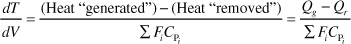
11.2.3 Overview of Energy Balances

What is the plan? In the following pages we manipulate Equation (11-9) in order to apply it to each of the reactor types we have been discussing: batch, PFR, PBR, and CSTR. The end result of the application of the energy balance to each type of reactor is shown in Table 11-1. These equations can be used in Step 5 of the algorithm discussed in Example E11-1. The equations in Table 11-1 relate temperature to conversion and to molar flow rates and to the system parameters, such as the overall heat-transfer coefficient and area, Ua, with the corresponding ambient temperature, T_a, and the heat of reaction, ΔH_Rx.

Example 11-1. Energy Balances of Common Reactors

1. Adiabatic CSTR, PFR, Batch, or PBR. The relationship between conversion, X_EB, and temperature for , constant C_Pi, and ΔC_P = 0, is
   

   T11-1.A

   

   T11-1.B

   

   End results of manipulating the energy balance (Sections 11.2.4, 12.1, and 12.3).

   For an exothermic reaction (–ΔH_Rx) > 0

   

2. CSTR with heat exchanger, UA (T_a – T), and large coolant flow rate.
   

   T11-1.C

   

3. PFR/PBR with heat exchange
   

   

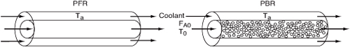
   In general most of the PFR and PBR energy balances can be written as

   

   3A. PFR in terms of conversion

   T11-1.D

   

   3B. PBR in terms of conversion

   T11-1.E

   

   3C. PBR in terms of molar flow rates

   T11-1.F

   

   3D. PFR in terms of molar flow rates

   T11-1.G

   

4. Batch
   

   T11-1.H

   

5. For Semibatch or unsteady CSTR
   

   T11-1.I

   

6. For multiple reactions in a PFR (q reactions and m species)
   

   T11-1.J

   

7. Variable heat exchange fluid temperature, T_a
   

   

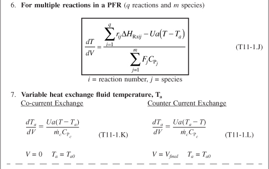
The equations in Table 11-1 are the ones we will use to solve reaction engineering problems with heat effects.

[Nomenclature: U = overall heat-transfer coefficient, (J/m² · s · K); A = CSTR heat-exchange area, (m²); a = PFR heat-exchange area per volume of reactor, (m²/m³); C_Pi = mean heat capacity of species i, (J/mol/K); C_Pc = the heat capacity of the coolant, (J/kg/K), = coolant flow rate, (kg/s); ΔH_Rx = heat of reaction, (J/mol);

ΔH_Rxij = heat of reaction wrt species j in reaction i, (J/mol);

= heat added to the reactor, (J/s); and

All other symbols are as defined in Chapters 5 and 6.]

Examples of How to Use Table 11-1. We now couple the energy balance equations in Table 11-1 with the appropriate reactor mole balance, rate law, and stoichiometry algorithm to solve reaction engineering problems with heat effects. For example, recall the rate law for a first-order reaction, Equation (E11-1.5) in Example 11-1.

E11-1.5

If the reaction is carried out adiabatically, then we use Equation (T11-1.B) for the reaction in Example 11-1 to obtain

T11-1.B

Consequently, we can now obtain –r_A as a function of X alone by first choosing X, then calculating T from Equation (T11-1.B), then calculating k from Equation (E11-1.3), and then finally calculating (–r_A) from Equation (E11-1.5).

We can use this sequence to prepare a table of (F_A0/–r_A) as a function of X. We can then proceed to size PFRs and CSTRs. In the absolute worst case scenario, we could use the techniques in Chapter 2 (e.g., Levenspiel plots or the quadrature formulas in Appendix A). However, instead of using a Levenspiel plot, we will most likely use Polymath to solve our coupled differential energy and mole balance equations.

If there is cooling along the length of a PFR, we could then apply Equation (T11-1.D) to this reaction to arrive at two coupled differential equations.

which are easily solved using an ODE solver such as Polymath.

Similarly, for the case of the reaction A → B carried out in a CSTR, we could use Polymath or MATLAB to solve two nonlinear algebraic equations in X and T. These two equations are the combined mole balance

and the application of Equation (T11-1.C), which is rearranged in the form

From these three cases, (1) adiabatic PFR and CSTR, (2) PFR and PBR with heat effects, and (3) CSTR with heat effects, one can see how one couples the energy balances and mole balances. In principle, one could simply use Table 11-1 to apply to different reactors and reaction systems without further discussion. However, understanding the derivation of these equations will greatly facilitate their proper application and evaluation to various reactors and reaction systems. Consequently, we now derive the equations given in Table 11-1.

Why bother to derive the equations in Table 11-1? Because I have found that students can apply these equations much more accurately to solve reaction engineering problems with heat effects if they have gone through the derivation to understand the assumptions and manipulations used in arriving at the equations in Table 11.1.

11.3 The User Friendly Energy Balance Equations

We will now dissect the molar flow rates and enthalpy terms in Equation (11-9) to arrive at a set of equations we can readily apply to a number of reactor situations.