
11.5.2 Reactor Staging
Reactor Staging with Interstage Cooling or Heating
Conversions higher than those shown in Figure E11-4.1 can be achieved for adiabatic operations by connecting reactors in series with interstage cooling:
Figure 11-5. Reactor in series with interstage cooling.
![]()
Exothermic Reactions
The conversion–temperature plot for this scheme is shown in Figure 11-6. We see that with three interstage coolers, 88% conversion can be achieved, compared to an equilibrium conversion of 35% for no interstage cooling.
Figure 11-6. Increasing conversion by interstage cooling for an exothermic reaction.

Endothermic Reactions
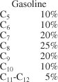
Another example of the need for interstage heat transfer in a series of reactors can be found when upgrading the octane number of gasoline. The more compact the hydrocarbon molecule for a given number of carbon atoms is, the higher the octane rating (see Section 10.3.5). Consequently, it is desirable to convert straight-chain hydrocarbons to branched isomers, naphthenes, and aromatics. The reaction sequence is
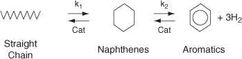
The first reaction step (K1) is slow compared to the second step, and each step is highly endothermic. The allowable temperature range for which this reaction can be carried out is quite narrow: Above 530°C undesirable side reactions occur, and below 430°C the reaction virtually does not take place. A typical feed stock might consist of 75% straight chains, 15% naphthas, and 10% aromatics.
One arrangement currently used to carry out these reactions is shown in Figure 11-7. Note that the reactors are not all the same size. Typical sizes are on the order of 10 m to 20 m high and 2 m to 5 m in diameter. A typical feed rate of gasoline is approximately 200 m3/h at 2 atm. Hydrogen is usually separated from the product stream and recycled.
Figure 11-7. Interstage heating for gasoline production in moving-bed reactors.

Because the reaction is endothermic, the equilibrium conversion increases with increasing temperature. A typical equilibrium curve and temperature conversion trajectory for the reactor sequence are shown in Figure 11-8.
Figure 11-8. Temperature–conversion trajectory for interstage heating of an endothermic reaction analogous to Figure 11-6.

Example 11-5. Interstage Cooling for Highly Exothermic Reactions
What conversion could be achieved in Example 11-4 if two interstage coolers that had the capacity to cool the exit stream to 350 K were available? Also, determine the heat duty of each exchanger for a molar feed rate of A of 40 mol/s. Assume that 95% of the equilibrium conversion is achieved in each reactor. The feed temperature to the first reactor is 300 K.
- Calculate Exit Temperature
We saw in Example 11-4

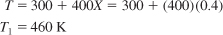
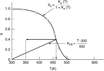
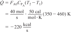
that for an entering temperature of 300 K the adiabatic equilibrium conversion was 0.42. For 95% of the equilibrium conversion (Xe = 0.42), the conversion exiting the first reactor is 0.4. The exit temperature is found from a rearrangement of Equation (E11-4.7):
We now cool the gas stream exiting the reactor at 460 K down to 350 K in a heat exchanger (Figure E11-5.2).
Figure E11-5.1. Determining exit conversion and temperature in the first stage.
- Calculate the Heat Load
There is no work done on the reaction gas mixture in the exchanger, and the reaction does not take place in the exchanger. Under these conditions (Fi|in = Fi|out), the energy balance given by Equation (11-10)

for
 becomes

But CPA = CPB,
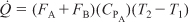
Also, for this example, FA0 = FA + FB,
That is, 220 kcal/s must be removed to cool the reacting mixture from 460 K to 350 K for a feed rate of 40 mol/s.
- Second Reactor
Now let’s return to determine the conversion in the second reactor. Rearranging Equation (E11-4.7) for the second reactor
The conditions entering the second reactor are T = 350 K and X = 0.4. The energy balance starting from this point is shown in Figure E11-5.2. The corresponding adiabatic equilibrium conversion is 0.63. Ninety-five percent of the equilibrium conversion is 60% and the corresponding exit temperature is T = 350 + (0.6 – 0.4)400 = 430 K.
- Heat Load
The heat-exchange duty to cool the reacting mixture from 430 K back to 350 K can again be calculated from Equation (E11-5.5):

- Subsequent Reactors
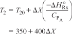
For the final reactor we begin at T0 = 350 K and X = 0.6 and follow the line representing the equation for the energy balance along to the point of intersection with the equilibrium conversion, which is X = 0.8. Consequently, the final conversion achieved with three reactors and two interstage coolers is (0.95)(0.8) = 0.76.
Figure E11-5.2. Three reactors in series with interstage cooling.
Analysis: For highly exothermic reactions carried out adiabatically, reactor staging with interstage cooling can be used to obtain high conversions. One observes that the exit conversion and temperature from the first reactor are 40% and 450 K respectively, as shown by the energy balance line. The exit stream at this conversion is then cooled to 350 K where it enters the second reactor. In the second reactor the overall conversion and temperature increase to 60% and 445 K. The slope of X versus T from the energy balance is the same as the first reactor. This example also showed how to calculate the heat load on each exchanger. We also note that the heat load on the third exchanger will be less than the first exchanger because the exit temperature from the second reactor (445 K) is lower than that the first reactor (450 K). Consequently, less heat needs to be removed by the third exchanger.
11.6 Optimum Feed Temperature
We now consider an adiabatic reactor of fixed size or catalyst weight and investigate what happens as the feed temperature is varied. The reaction is reversible and exothermic. At one extreme, using a very high feed temperature, the specific reaction rate will be large and the reaction will proceed rapidly, but the equilibrium conversion will be close to zero. Consequently, very little product will be formed. At the other extreme of low feed temperatures, little product will be formed because the reaction rate is so low. A plot of the equilibrium conversion and the conversion calculated from the adiabatic energy balance is shown in Figure 11-9. Substituting into Equation (T11-1.A) for the case where ![]() , the energy balance line shown in Figure 11-9 is XEB = 0.069(T – T0). We see that for an entering temperature of 600 K the adiabatic equilibrium conversion is 0.15, while for an entering temperature of 350K it is 0.75. The corresponding conversion profiles down the length of the reactor for these temperatures are shown in Figure 11-10. The equilibrium conversion, which can be calculated from Equation (E11-4.2) for a first order reaction also varies along the length of the reactor, as shown by the dashed line in Figure 11-10. We also see that because of the high entering temperature, the rate is very rapid at the inlet and equilibrium is achieved very near the reactor entrance.
, the energy balance line shown in Figure 11-9 is XEB = 0.069(T – T0). We see that for an entering temperature of 600 K the adiabatic equilibrium conversion is 0.15, while for an entering temperature of 350K it is 0.75. The corresponding conversion profiles down the length of the reactor for these temperatures are shown in Figure 11-10. The equilibrium conversion, which can be calculated from Equation (E11-4.2) for a first order reaction also varies along the length of the reactor, as shown by the dashed line in Figure 11-10. We also see that because of the high entering temperature, the rate is very rapid at the inlet and equilibrium is achieved very near the reactor entrance.
Figure 11-9. Equilibrium conversion for different feed temperatures.

Figure 11-10. Adiabatic conversion profiles for different feed temperatures.
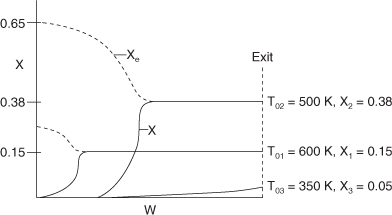
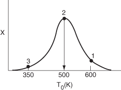
We notice that the conversion and temperature increase very rapidly over a short distance (i.e., a small amount of catalyst). This sharp increase is sometimes referred to as the “point” or temperature at which the reaction “ignites.” If the inlet temperature were lowered to 500 K, the corresponding equilibrium conversion would increase to 0.38; however, the reaction rate is slower at this lower temperature so that this conversion is not achieved until closer to the end of the reactor. If the entering temperature were lowered further to 350 K, the corresponding equilibrium conversion would be 0.75, but the rate is so slow that a conversion of 0.05 is achieved for the specified catalyst weight in the reactor. At a very low feed temperature, the specific reaction rate will be so small that virtually all of the reactant will pass through the reactor without reacting. It is apparent that with conversions close to zero for both high and low feed temperatures, there must be an optimum feed temperature that maximizes conversion. As the feed temperature is increased from a very low value, the specific reaction rate will increase, as will the conversion. The conversion will continue to increase with increasing feed temperature until the equilibrium conversion is approached in the reaction. Further increases in feed temperature for this exothermic reaction will only decrease the conversion due to the decreasing equilibrium conversion. This optimum inlet temperature is shown in Figure 11-11.
Figure 11-11. Finding the optimum feed temperature.
Summary
For the reaction
![]()
- The heat of reaction at temperature T, per mole of A, is

- The mean heat capacity difference, ΔCP, per mole of A is
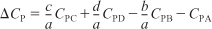
where CPi is the mean heat capacity of species i between temperatures TR and T.
- When there are no phase changes, the heat of reaction at temperature T is related to the heat of reaction at the standard reference temperature TR by

- The steady state energy balance on a system volume V is

- For adiabatic operation
 of a PFR, PBR, CSTR, or batch reactor, and neglecting
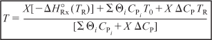
  , we solve Equation (S11-4) for the adiabatic conversion-temperature relationship is:
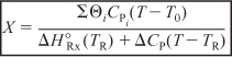
Solving Equation (S11-5) for the adiabatic temperature-conversion relationship:
DVD-ROM Material
• Learning Resources
- Summary Notes
- PFR/PBR Solution Procedure for a Reversible Gas-Phase Reaction

• Living Example Problems
- Example 11-3 Polymath Adiabatic Isomerization of Normal Butane
- Example 11-3 Formulated in AspenTech—Load from DVD-ROM

A step-by-step AspenTech tutorial is given on the DVD-ROM.
• Professional Reference Shelf
R11.1.
Variable Heat Capacities. Next we want to arrive at a form of the energy balance for the case where heat capacities are strong functions of temperature over a wide temperature range. Under these conditions, the mean values of the heat capacity may not be adequate for the relationship between conversion and temperature. Combining the heat of reaction with the quadratic form of the heat capacity,
CPi = αi + βiT + γiT2

we find that
![]()
Example 11-4 is reworked for the case of variable heat capacities.
Questions and Problems
The subscript to each of the problem numbers indicates the level of difficulty: A, least difficult; D, most difficult.
![]()

In each of the questions and problems, rather than just drawing a box around your answer, write a sentence or two describing how you solved the problem, the assumptions you made, the reasonableness of your answer, what you learned, and any other facts that you want to include. See the Preface for additional generic parts (x), (y), (z) to the home problems.

Read over the problems at the end of this chapter. Make up an original problem that uses the concepts presented in this chapter. To obtain a solution:
a. Make up your data and reaction.
b. Use a real reaction and real data. See Problem P5-1A for guidelines.
c. Prepare a list of safety considerations for designing and operating chemical reactors. What would be the first four items on your list? (See www.sache.org and www.siri.org/graphics.) The August 1985 issue of Chemical Engineering Progress may be useful.
d. Read through the Self Tests and Self Assessments for Chapter 11 on the DVD-ROM, and pick one that was most difficult.
e. Which example on the DVD-ROM Lecture Notes for Chapter 11 was the most difficult?
f. What if you were asked to give an everyday example that demonstrates the principles discussed in this chapter? (Would sipping a teaspoon of Tabasco or other hot sauce be one?)
g. Rework Problem P2-11B (page 69) for the case of adiabatic operation.
Load the following Polymath programs from the DVD-ROM where appropriate:
a. Example 11-1. How would this example change if a CSTR were used instead of a PFR?

b. Example 11-2. What would the heat of reaction be if 50% inerts (e.g., helium) were added to the system? What would be the % error if the ΔCP term were neglected?
c. Example 11-3. What if the butane reaction were carried out in a 0.8-m3 PFR that can be pressurized to very high pressures? What inlet temperature would you recommend? Is there an optimum inlet temperature? Plot the heat that must be removed along the reactor [![]() vs. V] to maintain isothermal operation.
vs. V] to maintain isothermal operation.
d. AspenTech Example 11-3. Load the AspenTech program from the DVD-ROM. (1) Repeat P11-2B (c) using AspenTech. (2) Vary the inlet flow rate and temperature and describe what you find.
e. Example 11-4. (1) Make a plot of the equilibrium conversion as a function of entering temperature, T0. (2) What do you observe at high and low T0? (3) Make a plot of Xe versus T0 when the feed is equal molar in inerts that have the same heat capacity. (4) Compare the plots of Xe versus T0 with and without inerts and describe what you find.
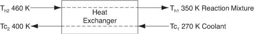
f. Example 11-5. (1) Determine the molar flow rate of cooling water (CPw = 18 cal/mol·K) necessary to remove 220 kcal/s from the first exchanger. The cooling water enters at 270 K and leaves at 400 K. (2) Determine the necessary heat exchanger area A (m2) for an overall heat transfer coefficient of 100 cal/s·m2·K. You must use the log-mean driving force in calculating A. [Hint: See DVD-ROM Summary Notes.]
E11-5.7
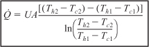
Figure . Figure P11-2B (e) Counter current heat exchanger.
The elementary irreversible organic liquid-phase reaction
A + B → C
is carried out adiabatically in a flow reactor. An equal molar feed in A and B enters at 27°C, and the volumetric flow rate is 2 dm3/s and CA0 = 0.1 kmol/m3.
Additional information:

a. Plot and then analyze the conversion and temperature as a function of PFR volume up to where X = 0.85. Describe the trends.
b. What is the maximum inlet temperature one could have so that the boiling point of the liquid (550 K) would not be exceeded even for complete conversion?
c. Plot the heat that must be removed along the reactor [![]() vs. V] to maintain isothermal operation.
vs. V] to maintain isothermal operation.
d. Plot and then analyze the conversion and temperature profiles up to a PFR reactor volume of 10 dm3 for the case when the reaction is reversible with KC = 10 m3/kmol at 450 K. Plot the equilibrium conversion profile. How are the trends different than part (a)?
The elementary irreversible gas-phase reaction
A → B + C
is carried out adiabatically in a PFR packed with a catalyst. Pure A enters the reactor at a volumetric flow rate of 20 dm3/s, at a pressure of 10 atm and a temperature of 450 K.
Additional information:
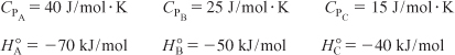
All heats of formation are referenced to 273 K.
![]()
a. Plot and then analyze the conversion and temperature down the plug-flow reactor until an 80% conversion (if possible) is reached. (The maximum catalyst weight that can be packed into the PFR is 50 kg.) Assume that ΔP = 0.0.
b. Vary the inlet temperature and describe what you find.
c. Plot the heat that must be removed along the reactor [![]() vs. V] to maintain isothermal operation.
vs. V] to maintain isothermal operation.
d. Now take the pressure drop into account in the PBR.
The reactor can be packed with one of two particle sizes. Choose one.
α = 0.019/kg cat. for particle diameter D1
α = 0.0075/kg cat. for particle diameter D2
e. Plot and then analyze the temperature, conversion, and pressure along the length of the reactor. Vary the parameters α and P0 to learn the ranges of values in which they dramatically affect the conversion.
f. Apply one or more of the six ideas in Table P-3, page xiii to this problem.
The irreversible endothermic vapor-phase reaction follows an elementary rate law
CH3COCH3 → CH2CO + CH4
A → B + C
and is carried out adiabatically in a 500-dm3 PFR. Species A is fed to the reactor at a rate of 10 mol/min and a pressure of 2 atm. An inert stream is also fed to the reactor at 2 atm, as shown in Figure P11-5B. The entrance temperature of both streams is 1100 K.
Figure . Figure P11-5B Adiabatic PFR with inerts.

Additional information:

a. First derive an expression for CA01 as a function of CA0 and ΘI.
b. Sketch the conversion and temperature profiles for the case when no inerts are present. Using a dashed line, sketch the profiles when a moderate amount of inerts are added. Using a dotted line, sketch the profiles when a large amount of inerts are added. Qualitative sketches are fine. Describe the similarities and differences between the curves.
c. Sketch or plot and then analyze the exit conversion as a function of ΘI. Is there a ratio of the entering molar flow rates of inerts (I) to A (i.e., ΘI = FI0/FA0) at which the conversion is at a maximum? Explain, why there “is” or “is not” a maximum.
d. What would change in parts (b) and (c) if reactions were exothermic and reversible with ![]() and KC = 2 dm3/mol at 1100 K?
and KC = 2 dm3/mol at 1100 K?
e. Sketch or plot FB for parts (c) and (d) and describe what you find.
f. Plot the heat that must be removed along the reactor [![]() vs. V] to maintain isothermal operation for pure A fed and an exothermic reaction.
vs. V] to maintain isothermal operation for pure A fed and an exothermic reaction.
The gas phase reversible reaction
A ⇄ B
is carried out under high pressure in a packed-bed reactor with pressure drop. The feed consists of both inerts I and Species A with the ratio of inerts to the species A being 2 to 1. The molar flow rate of A is 5 mol/min at a temperature of 300 K and a concentration of 2 mol/dm3. Work this problem in terms of volume [Hint: V = W/ρB, ![]() ].
].
Additional information:

a. Adiabatic Operation. Plot X, Xe, T and the rate of disappearance as a function of V up to V = 40 dm3. Explain why the curves look the way they do.
b. Vary the ratio of inerts to A (0 ≤ ΘI ≤ 10) and the entering temperature and describe what you find.
c. Plot the heat that must be removed along the reactor [![]() vs. V] to maintain isothermal operation.
vs. V] to maintain isothermal operation.
We will continue this problem in Chapter 12.
Algorithm for reaction in a PBR with heat effects
The Elementary Gas Phase Reaction
![]()
is carried out in a packed-bed reactor. The entering molar flow rates are FA0 = 5 mol/s, FB0 = 2FA0, F1 = 2FA0 with CA0 = 0.2 mol/dm3. The entering temperature is 325 K and a coolant fluid is available at 300 K.
Additional information:
a. Write the mole balance, the rate law, KC as a function of T, k as a function of T and CA, CB, CC as a function of X, y and T.
b. Write the rate law as a function of X, y, and T.
c. Show the equilibrium conversion is

d. What are ΣΘiCPi, ΔCP, T0, entering temperature T1 (rate law) and T2 (equilibrium constant)?
e. Write the energy balance for adiabatic operation.
f. Case 1 Adiabatic Operation. Plot and then analyze Xe, X, y, and T versus W when the reaction is carried out adiabatically. Describe why the profiles look the way they do. Identify those terms which will be affected by inerts. Sketch what you think the profiles Xe, X, y, and T will look like before you run the Polymath program to plot the profiles.
g. Plot the heat that must be removed along the reactor [![]() vs. V] to maintain isothermal operation.
vs. V] to maintain isothermal operation.
The reaction
![]()
is carried out adiabatically in a series of staged packed-bed reactors with interstage cooling (see Figure 11-5). The lowest temperature to which the reactant stream may be cooled is 27°C. The feed is equal molar in A and B and the catalyst weight in each reactor is sufficient to achieve 99.9% of the equilibrium conversion. The feed enters at 27°C and the reaction is carried out adiabatically. If four reactors and three coolers are available, what conversion may be achieved?
Additional information:
![]()
First prepare a plot of equilibrium conversion as a function of temperature. [Partial ans.: T = 360 K, Xe = 0.984; T = 520 K, Xe = 0.09; T = 540 K, Xe = 0.057]
Figure P11-9 shows the temperature-conversion trajectory for a train of reactors with interstage heating. Now consider replacing the interstage heating with injection of the feed stream in three equal portions, as shown in Figure P11-9:

Sketch the temperature-conversion trajectories for (a) an endothermic reaction with entering temperatures as shown, and (b) an exothermic reaction with the temperatures to and from the first reactor reversed, i.e., T0 = 450°C.
What’s wrong with this solution?
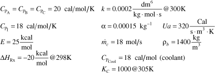
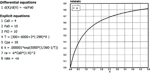
The liquid phase elementary reaction
![]()
is carried out adiabatically in a 5 dm3 PFR. The heat of reaction at 298 K is –10,000 cal/mol A. The feed is equal molar in A and in inerts at 77°C, with FA = 10 mol/min and CA0 = 4 mol/dm3.
Plot X as a function of reactor volume.
Additional information:
CPA = 18 cal/mol, CPB = CPC = 9 cal/mol, and CPInerts = 15 cal/mol
k = 10-6 dm3/mol•min at 360 K with E = 6,000 cal/mol
Solution
Taking A as our basis of calculation and dividing through by the stoichiometric coefficient 2,
![]()
the heat of reaction at 298 K per mole of our basis of calculation is thus:

The Polymath solution is shown below
Figure . Figure P11-10B Polymath program and graphical output.
Supplementary Reading
- An excellent development of the energy balance is presented in
ARIS, R., Elementary Chemical Reactor Analysis. Upper Saddle River, N.J.: Prentice Hall, 1969, Chaps. 3 and 6.
A number of example problems dealing with nonisothermal reactors can be found in
BURGESS, THORNTON W., The Adventures of Old Man Coyote. New York: Dover Publications, Inc., 1916.
BUTT, JOHN B., Reaction Kinetics and Reactor Design, Revised and Expanded, 2nd ed. New York: Marcel Dekker, Inc., 1999.
WALAS, S.M., Chemical Reaction Engineering Handbook of Solved Problems, Amsterdam: Gordon and Breach, 1995. See the following solved problems: 4.10.1, 4.10.08, 4.10.09, 4.10.13, 4.11.02, 4.11.09, 4.11.03, 4.10.11.
For a thorough discussion on the heat of reaction and equilibrium constant, one might also consult
DENBIGH, K. G., Principles of Chemical Equilibrium, 4th ed. Cambridge: Cambridge University Press, 1981.
- The heats of formation, Hi(T), Gibbs free energies, Gi(TR), and the heat capacities of various compounds can be found in
GREEN, D. W. and R. H. PERRY, eds., Chemical Engineers’ Handbook, 8th ed. New York: McGraw-Hill, 2008.
REID, R. C., J. M. PRAUSNITZ, and T. K. SHERWOOD, The Properties of Gases and Liquids, 3rd ed. New York: McGraw-Hill, 1977.
WEAST, R. C., ed., CRC Handbook of Chemistry and Physics, 66th ed. Boca Raton, Fla.: CRC Press, 1985.