
12.3.1 Applying the Algorithm to an Exothermic Reaction
Example 12-1. Butane Isomerization Continued—OOPS!
When we checked the vapor pressure at the exit to the adiabatic reactor in Example 11-3 where the temperature is 360 K, we found the vapor pressure to be about 1.5 MPa for isobutene, which is greater than the rupture pressure of the glass vessel being used. Fortunately, there is a bank of 10 tubular reactors, each reactor is 5 m3. The bank reactors are double pipe heat exchangers with the reactants flowing in the inner pipe and with Ua = 5,000 kJ/m3·h·K. The entering temperature of the reactants is 305 K and the entering coolant temperature is 310 K. The mass flow rate of the coolant, ![]() , is 500 kg/h and the heat capacity of the coolant, CPC, is 28 kJ/kg·K. The temperature in any one of the reactors cannot rise above 325 K. Carry out the following analyses:
, is 500 kg/h and the heat capacity of the coolant, CPC, is 28 kJ/kg·K. The temperature in any one of the reactors cannot rise above 325 K. Carry out the following analyses:
a. Co-current heat exchange. Plot X, Xe, T, Ta, and –rA, down the length of the reactor.
b. Counter current heat exchange. Plot X, Xe, T, Ta, and –rA down the length of the reactor.
c. Constant ambient temperature, Ta. Plot X, Xe, T, and –rA down the length of the reactor.
d. Compare parts (a), (b), and (c) above with the adiabatic case discussed in Example 11-3. Write a paragraph describing what you find.
Additional information
Recall from Example 11-3 that CPA 141 kJ/kmol · K, CP0 ΣΘiCPi = 159 kJ/kmol · K, ΔHRx = –6,900 kJ/kmol, and ΔCP = 0.
We shall first solve Part (a), the co-current heat exchange case first and then make small changes in the Polymath program for Parts (b) through (d).
For each of the ten reactors in parallel
![]()
The mole balance, rate law, and stoichiometry are the same as in the adiabatic case previously discussed in Example 11-3; that is,
Same as Example 11-3
Mole Balance:
![]()
Rate Law and Stoichiometry:

with
![]()
![]()
The equilibrium conversion is
![]()
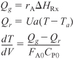
The energy balance on the reactor is

Part (a) Co-Current Heat Exchange
For co-current flow, the balance on the heat transfer fluid is

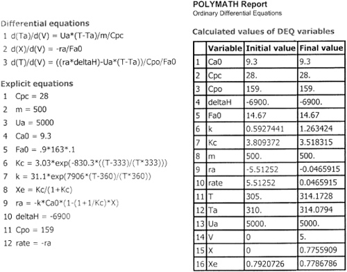
with Ta = 310 K at V = 0. The Polymath program and solution are shown in Table E12-1.1.
Table E12-1.1. PART (a) Co-current Heat Exchange

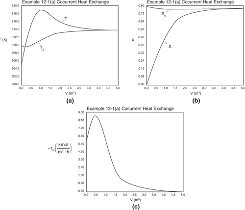
Analysis: Part (a) Co-Current Exchange: We note that reactor temperature goes through a maximum. Near the reactor entrance, the reactant concentrations are high and therefore the reaction rate is high [c.f. Figure E12-1.1(a)] and Qg > Qr. Consequently, the temperature increases with increasing reactor volume. However, further down the reactor, the reactants have been mostly consumed, the rate is small Qr > Qg, and the temperature decreases. We also note that when the ambient heat exchanger temperature and the reactor temperature are essentially equal, there is no longer a temperature driving force to cool the reactor. Consequently, the temperature does not change further down the reactor, nor does the equilibrium conversion, which is only a function of temperature.
Figure E12-1.1. Profiles down the reactor for co-current heat exchange (a) temperature, (b) conversion, (c) reaction rate.
Part (b) Counter Current Heat Exchange:
For counter current flow we only need to make two changes in the program. First, multiply the right hand side of Equation (E12-1.2) by minus one to obtain
![]()
Next, we guess Ta at V = 0 and see if it matches Ta0 at V = 5 m3. If it doesn’t, we guess again. In this example, we will guess Ta (V = 0) = 315 K and see if Ta = Ta0 = 310 K at V = 5 m3.
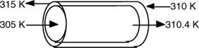
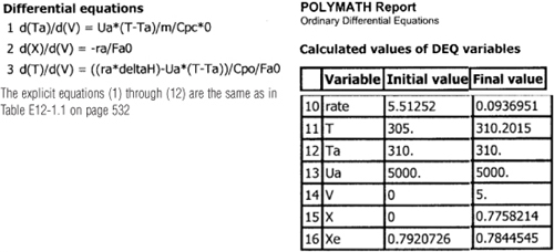
Table E12-1.2. Part (b) Counter Current Heat Exchange

What a lucky guess we made of 315 K at V = 0 to find Ta0 = 310!! The variable profiles are shown in Figure E12-1.2.
Figure E12-1.2. Profiles down the reactor for counter current heat exchange (a) temperature, (b) conversion, (c) reaction rate.
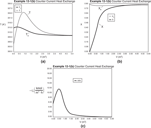
Analysis: Part (b) Counter Current Exchange: We note that near the entrance to the reactor, the coolant temperature is above the reactant entrance temperature. However, as we move down the reactor the reaction generates “heat” and the reactor temperature rises above the coolant temperature. We note that Xe reaches a minimum (corresponding to the reactor temperature maximum) near the entrance to the reactor and then increases as the reactor temperature decreases. A higher maximum temperature in the reactor, along with a higher exit conversion, X, and equilibrium conversion, Xe, are achieved in the counter current heat exchange system than for the co-current system.
For constant Ta, use the Polymath program in Part (a), but multiply the right side of Equation (E12-1.2) by zero in the program, i.e.,
![]()
Table E12-1.3. Part (c) Constant Ta
The initial and final values are shown in the Polymath report and the variable profiles are shown in Figure E12-1.3.
Figure E12-1.3. Profiles down the reactor for constant heat exchange fluid temperature Ta (a) temperature, (b) conversion, (c) reaction rate.

Analysis: Part (c) Constant Ta: When the coolant flow rate is sufficiently large, the coolant temperature Ta will be essentially constant. If the reactor volume is sufficiently large, the reactor temperature will eventually reach the coolant temperature, as is the case here. At this exit temperature, which the lowest achieved in this example, the equilibrium conversion Xe is the largest of the four cases studied in this example.
Part (d) Adiabatic Operation
In Example 11-3, we solved for the temperature as a function of conversion and then used that relationship to calculate k and KC. An easier way is to solve the general or base case of a heat exchanger for co-current flow and write the corresponding Polymath program. Next use Polymath [Part (a)], but multiply the parameter Ua by zero, i.e.,
Ua = 5,000 * 0
Table E12-1.4. Part (d) Adiabatic Operation

The initial and exit conditions are shown in the Polymath report, while the profiles of T, X, Xe, and –rA are shown in Figure E12-1.4.
Figure E12-1.4. Profiles down the reactor for adiabatic reactor (a) temperature, (b) conversion, (c) reaction rate.
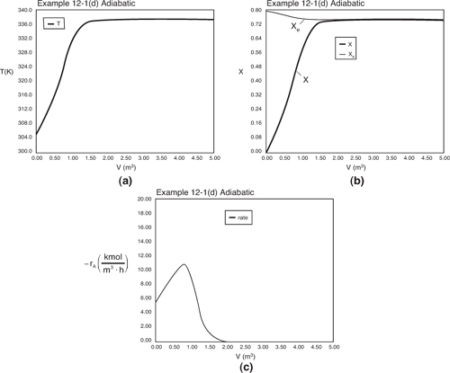
Analysis: Part (d) Adiabatic Operation: Because there is no cooling, the reactor temperature reaches the highest temperature and lowest equilibrium conversion of the four cases considered in this example, i.e., the adiabatic equilibrium temperature and conversion. In fact, these values are reached after 2 m3 down the reactor, so the remaining volume after this point up to 5 m3 serves no purpose. When comparing the conversion reached in the adiabatic case (X = 0.746) with the conversion for the reactors with heat exchangers (ca X = 0.78) one has to ask the question, “Is the cost of a heat exchange system justified?” If side reactions occur at this higher temperature, the answer is yes.
Overall Analysis: This is an extremely important example, as we applied our CRE PFR algorithm with heat exchange to a reversible exothermic reaction. We analyzed four types of heat exchanger operations. We see the counter current exchanger gives the highest conversion and adiabatic operation gives the lowest conversion. Equilibrium is reached the earliest (1.5 m3) in the adiabatic reactors and the latest in the reactors where Ta is constant.