
12.4.1 Heat Added to the Reactor, 
Figure 12-6 shows schematics of a CSTR with a heat exchanger. The heat transfer fluid enters the exchanger at a mass flow rate ![]() (e.g., kg/s) at a temperature Ta1 and leaves at a temperature Ta2. The rate of heat transfer from the exchanger to the reactor fluid at temperature T is3
(e.g., kg/s) at a temperature Ta1 and leaves at a temperature Ta2. The rate of heat transfer from the exchanger to the reactor fluid at temperature T is3
![]()
Figure 12-6. CSTR tank reactor with heat exchanger.
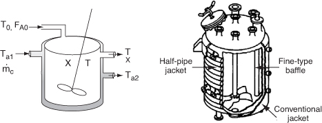
Diagram on right courtesy of Pfaudler, Inc.
The following derivations, based on a coolant (exothermic reaction) apply also to heating mediums (endothermic reaction). As a first approximation, we assume a quasi-steady state for the coolant flow and neglect the accumulation term (i.e., dTa/dt = 0). An energy balance on the heat exchanger fluid entering and leaving the exchanger is

![]()
where CPc is the heat capacity of the heat exchanger fluid and TR is the reference temperature. Simplifying gives us
![]()
Solving Equation (12-16) for the exit temperature of the heat exchanger fluid yields
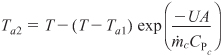
From Equation (12-16)
![]()
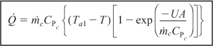
Substituting for Ta2 in Equation (12-18), we obtain
For large values of the heat exchanger fluid flow rate, the exponent will be small and can be expanded in a Taylor series (e–x = 1 – x + . . .) where second-order terms are neglected in order to give
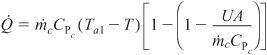
Then
![]()
where Ta1 ≅ Ta2 = Ta.
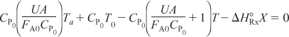
With the exception of processes involving highly viscous materials such as Problem P12-6B, a California Professional Engineers’ Exam Problem, the work done by the stirrer can usually be neglected. Setting ![]() in (11-27) to zero, neglecting ΔCP, substituting for
in (11-27) to zero, neglecting ΔCP, substituting for ![]() and rearranging, we have the following relationship between conversion and temperature in a CSTR.
and rearranging, we have the following relationship between conversion and temperature in a CSTR.
![]()
Solving for X:

Equation (12-22) is coupled with the mole balance equation

to design CSTRs.
We now will further rearrange Equation (12-21) after letting
![]()
then
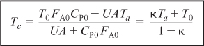
Let κ and TC be non-adiabatic parameters defined by

Then
![]()
The parameters κ and Tc are used to simplify the equations for non-adiabatic operation. Solving Equation (12-24) for conversion:
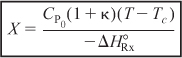
Solving Equation (12-24) for the reactor temperature:

Table 12-3 shows three ways to specify the design of a CSTR. This procedure for non-isothermal CSTR design can be illustrated by considering a first-order irreversible liquid-phase reaction. The algorithm for working through either cases A (X specified), B (T specified), or C (V specified) is shown in Table 12-3. Its application is illustrated in Example 12-3.
Table 12-3. Ways to Specify the Sizing of a CSTR

Example 12-3. Production of Propylene Glycol in an Adiabatic CSTR
Propylene glycol is produced by the hydrolysis of propylene oxide:

Over 900 million pounds of propylene glycol were produced in 2010 and the selling price was approximately $0.80 per pound. Propylene glycol makes up about 25% of the major derivatives of propylene oxide. The reaction takes place readily at room temperature when catalyzed by sulfuric acid.
You are the engineer in charge of an adiabatic CSTR producing propylene glycol by this method. Unfortunately, the reactor is beginning to leak, and you must replace it. (You told your boss several times that sulfuric acid was corrosive and that mild steel was a poor material for construction. He wouldn’t listen.) There is a nice-looking, shiny overflow CSTR of 300-gal capacity standing idle; it is glass-lined, and you would like to use it.
We are going to work this problem in lbm, s, ft3 and lb-moles rather than g, mol, and m3 in order to give the reader more practice in working in both the English and metric systems. Many plants still use the English system of units.
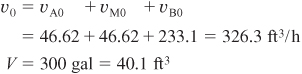
You are feeding 2500 lbm/h (43.04 lb-mol/h) of propylene oxide (P.O.) to the reactor. The feed stream consists of (1) an equivolumetric mixture of propylene oxide (46.62 ft3/h) and methanol (46.62 ft3/h), and (2) water containing 0.1 wt % H2SO4. The volumetric flow rate of water is 233.1 ft3/h, which is 2.5 times the methanol–P.O. volumetric flow rate. The corresponding molar feed rates of methanol and water are 71.87 lb-mol/h and 802.8 lb-mol/h, respectively. The water–propylene oxide–methanol mixture undergoes a slight decrease in volume upon mixing (approximately 3%), but you neglect this decrease in your calculations. The temperature of both feed streams is 58°F prior to mixing, but there is an immediate 17°F temperature rise upon mixing of the two feed streams caused by the heat of mixing. The entering temperature of all feed streams is thus taken to be 75°F (Figure E12-3.1).
Figure E12-3.1. Propylene Glycol manufacture in a CSTR.

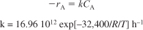
Furusawa et al.4 state that under conditions similar to those at which you are operating, the reaction is first-order in propylene oxide concentration and apparent zero-order in excess of water with the specific reaction rate
k = Ae–E/RT = 16.96 × 10¹²(e–32,400/RT)h–1
The units of E are Btu/lb-mol and T is in °R.
There is an important constraint on your operation. Propylene oxide is a rather low-boiling point substance. With the mixture you are using, you feel that you cannot exceed an operating temperature of 125°F, or you will lose too much oxide by vaporization through the vent system.
a. Can you use the idle CSTR as a replacement for the leaking one if it will be operated adiabatically?
b. If so, what will be the conversion of propylene oxide to glycol?
(All data used in this problem were obtained from the Handbook of Chemistry and Physics unless otherwise noted.) Let the reaction be represented by
![]()
where
A is propylene oxide (CPA = 35 Btu/lb-mol · °F)5
B is water (CPB = 18 Btu/lb-mol · °F)
C is propylene glycol (CPC = 46 Btu/lb-mol · °F)
M is methanol (CPM = 19.5 Btu/lb-mol · °F)
In this problem, neither the exit conversion nor the temperature of the adiabatic reactor is given. By application of the mole and energy balances, we can solve two equations with two unknowns (X and T), as shown on the right-hand pathway in Table 12-3. Solving these coupled equations, we determine the exit conversion and temperature for the glass-lined reactor to see if it can be used to replace the present reactor.
- Mole Balance and Design Equation:
FA0 – FA + rAV = 0
The design equation in terms of X is

- Rate Law:

- Stoichiometry (liquid phase, υ = υ0):
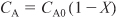
- Combining yields
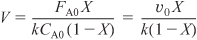
Solving for X as a function of T and recalling that τ = V/υ0 gives
This equation relates temperature and conversion through the mole balance.
- The energy balance for this adiabatic reaction in which there is negligible energy input provided by the stirrer is
This equation relates X and T through the energy balance. We see that two equations [Equations (E12-3.5) and (E12-3.6)] must be solved with XMB = XEB for the two unknowns, X and T.
- Calculations:
a. Evaluate the mole balance terms (CA0, Θi, τ): The total liquid volumetric flow rate entering the reactor is
E12-3.7
E12-3.8
E12-3.9
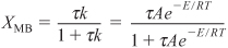
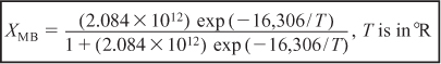
The conversion calculated from the mole balance, XMB, is found from Equation (E12-3.5).

E12-3.10
b. Evaluating the energy balance terms
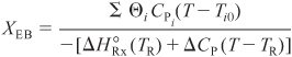
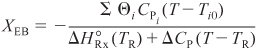
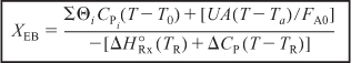
The conversion calculated from the energy balance, XEB, for an adiabatic reaction is given by Equation (11-29):
Substituting all the known quantities into the energy balance gives us

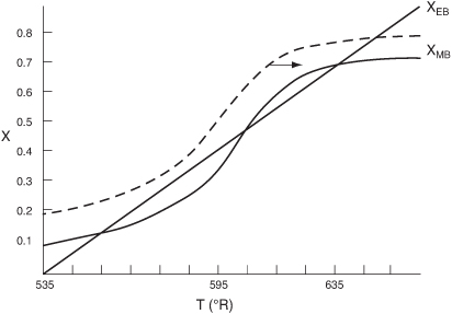
- Solving. There are a number of different ways to solve these two simultaneous algebraic equations (E12-3.10) and (E12-3.14). The easiest way is to use the Polymath nonlinear equation solver. However, to give insight into the functional relationship between X and T for the mole and energy balances, we shall obtain a graphical solution. Here X is plotted as a function of T for both the mole and energy balances, and the intersection of the two curves gives the solution where both the mole and energy balance solutions are satisfied i.e., XEB = XMB. In addition, by plotting these two curves we can learn if there is more than one intersection (i.e., multiple steady states) for which both the energy balance and mole balance are satisfied. If numerical root-finding techniques were used to solve for X and T, it would be quite possible to obtain only one root when there is actually more than one. If Polymath were used, you could learn if multiple roots exist by changing your initial guesses in the nonlinear equation solver. We shall discuss multiple steady states further in Section 12-4. We choose T and then calculate X (Table E12-3.1). The calculations for XMB and XEB are plotted in Figure E12-3.2. The virtually straight line corresponds to the energy balance [Equation (E12-3.14)] and the curved line corresponds to the mole balance [Equation (E12-3.10)]. We observe from this plot that the only intersection point is at 83% conversion and 613°R. At this point, both the energy balance and mole balance are satisfied. Because the temperature must remain below 125°F (585°R), we cannot use the 300-gal reactor as it is now.
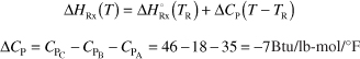


Table E12-3.1. Calculations of XEB and XMB as a Function of T

Figure E12-3.2. The conversions XEB and XMB as a function of temperature.
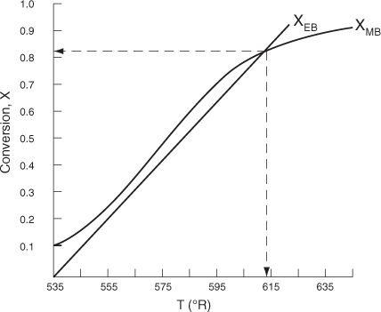
Analysis: We see that there is only one intersection of XEB(T) and XMB(T) and consequently only one steady state. The exit conversion is 83% and the exit temperature (i.e., the reactor temperature) is 613°R (153°F), which is above the acceptable limit of 585°R (125°F).
Oops! Looks like our plant will not be able to be completed and our multimillion dollar profit has flown the coop. But wait, don’t give up, let’s ask Fred to look in the storage shed. See what Fred found in Example 12-4.
Example 12-4. CSTR with a Cooling Coil
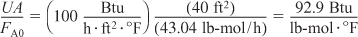
Fantastic! Fred has located a cooling coil in equipment storage for use in the hydrolsis of propylene oxide discussed in Example 12-3. The cooling coil has 40 ft2 of cooling surface and the cooling water flow rate inside the coil is sufficiently large that a constant coolant temperature of 85°F can be maintained. A typical overall heat-transfer coefficient for such a coil is 100 Btu/h·ft2·°F. Will the reactor satisfy the previous constraint of 125°F maximum temperature if the cooling coil is used?
If we assume that the cooling coil takes up negligible reactor volume, the conversion calculated as a function of temperature from the mole balance is the same as that in Example 12-3 [Equation (E12-3.11)].
- Combining the mole balance, stoichiometry, and rate law, we have, from Example 12-3,

T is in °R.
- Energy balance. Neglecting the work by the stirrer, we combine Equations (11-27) and (12-20) to write

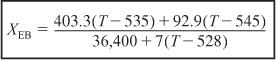
Solving the energy balance for XEB yields
The cooling coil term in Equation (E12-4.2) is
Recall that the cooling temperature is
Ta = 85°F = 545°R
The numerical values of all other terms of Equation (E12-4.2) are identical to those given in Equation (E12-3.13), but with the addition of the heat exchange term XEB becomes,
We now have two equations [(E12-3.10) and (E12-4.4)] and two unknowns, X and T, which we can solve with Polymath. Recall Examples E4-5 and E8-6 to review how to solve nonlinear, simultaneous equations of this type with Polymath.
Table E12-4.1. Polymath: CSTR with Heat Exchange

The POLYMATH program and solution to these two Equations (E12-3.10) for XMB, and (E12-4.4) for XEB, are given in Table E12-4.1. The exiting temperature and conversion are 103.7°F (563.7°R) and 36.4%, respectively, i.e.,
T = 564°R and X = 0,36
Analysis: By adding heat exchange to the CSTR, the XMB(T) curve is unchanged but the slope of XEB(T) line in Figure E12-3.2 increases and intersects the XMB curve at X = 0.36 and T = 564°R. This conversion is low! We could try to reduce to cooling by increasing Ta or T0 to raise the reactor temperature closer to 585°R, but not above this temperature. The higher the temperature in this irreversible reaction, the greater the conversion.
We will see in the next section that there may be multiple exit values of conversion and temperature (Multiple Steady States) that satisfy the parameter values and entrance conditions.
12.5 Multiple Steady States (MSS)
In this section we consider the steady-state operation of a CSTR in which a first-order reaction is taking place. An excellent experimental investigation that demonstrates the multiplicity of steady states was carried out by Vejtasa and Schmitz.6 They studied the reaction between sodium thiosulfate and hydrogen peroxide,
2Na2S2O3 + 4H2O2 → Na2SO4 + 4H2O
in a CSTR operated adiabatically. The multiple steady-state temperatures were examined by varying the flow rate over a range of space times, τ.
Reconsider the XMB(T) [Equation E12-3.10] curve shown in Figure E12-3.2, which has been re-drawn and shown as dashed lines in Figure E12-3.2A. Now consider what would happen if the volumetric flow rate υ0 is increased (τ decreased) just a little. The energy balance line XEB(T) remains unchanged, but the mole balance line XMB moves to the right, as shown by the curved, solid line in Figure E12-3.2A. This shift of XMB(T) to the right results in the XEB(T) and XMB(T) intersecting three lines, indicating three possible conditions at which the reactor can operate.
Figure E12-3.2A. Plots of XEB(T) and XMB(T) for different spaces times τ.
When more than one intersection occurs, there is more than one set of conditions that satisfy both the energy balance and mole balance (i.e., XEB = XMB), consequently, there will be multiple steady states at which the reactor may operate. These three steady states are easily determined from a graphical solution, but only one could show up in the Polymath solution. Consequently, when using the Polymath nonlinear equation solver we need to either choose different initial guesses to find if there are other solutions, or plot XMB and XEB versus T, as in Example 12-3.
We begin by recalling Equation (12-24), which applies when one neglects shaft work and ΔCP (i.e., ΔCP = 0 and therefore ![]() ).
).
![]()
where
![]()

and
Using the CSTR mole balance ![]() , Equation (12-24) may be rewritten as
, Equation (12-24) may be rewritten as
![]()
The left-hand side is referred to as the heat-generated term:
![]()
The right-hand side of Equation (12-28) is referred to as the heat-removed term (by flow and heat exchange) R(T):
![]()
To study the multiplicity of steady states, we shall plot both R(T) and G(T) as a function of temperature on the same graph and analyze the circumstances under which we will obtain multiple intersections of R(T) and G(T).