
12.6.4 Series Reactions in a CSTR
Example 12-6. Multiple Reactions in a CSTR
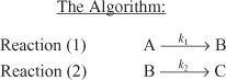
The elementary liquid-phase reactions
![]()
take place in a 10-dm3 CSTR. What are the effluent concentrations for a volumetric feed rate of 1000 dm3/min at a concentration of A of 0.3 mol/dm3?
The inlet temperature is 283 K.
CPA = CPB = CPC = 200 J/mol · K
k1 = 3.3 min–1 at 300 K, with E1 = 9900 cal/mol
k2 = 4.58 min–1 at 500 K, with E2 = 27,000 cal/mol
ΔHRx1A = –55,000 J/mol A
UA = 40,000 J/min · K with Ta = 57°C
ΔHRx2B = –71,500 J/mol B
The reactions follow elementary rate laws
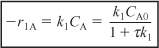
r1A = –k1ACA ≡ –k1CA
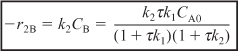
r2B = –k2BCB ≡ –k2CB
- Mole Balance on Every Species
Species A: Combined mole balance and rate law for A:

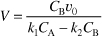
Solving for CA gives us

Species B: Combined mole balance and rate law for B:
Relative Rates
r1B = –r1A = k1CA
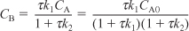
substituting for r1B and r2B in Equation (E12-6.3) gives
Solving for CB yields
- Rate Laws:
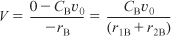
- Energy Balances:
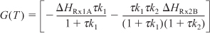
Applying Equation (12-41) to this system gives


Substituting for FA0 = υ0CA0, r1A, and r2B and rearranging, we have


We are going to generate G(T) and R(T) by fooling Polymath to first generate T as a function of a dummy variable, t. We then use our plotting options to convert T(t) to G(T) and R(T). The Polymath program to plot R(T) and G(T) vs. T is shown in Table E12-6.1, and the resulting graph is shown in Figure E12-6.1.
Table E12-6.1. Polymath Program and Output
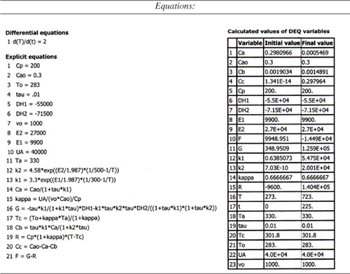

Figure E12-6.1. Heat-removed and heat-generated curves.
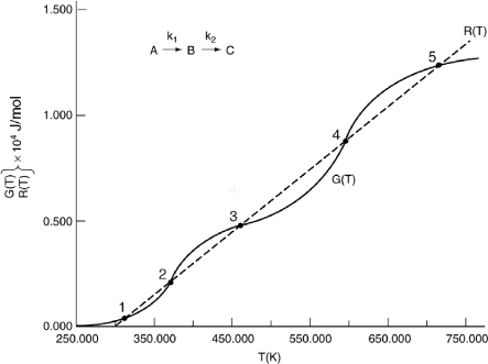
Table E12-6.2. Effluent Concentrations and Temperatures
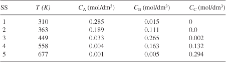
Analysis: Wow! We see that five steady states (SS) exist!! The exit concentrations and temperatures listed in Table E12-6.2 were determined from the tabular output of the Polymath program. Steady states 1, 3 and 5 are stable steady states, while 2 and 4 are unstable. The selectivity at steady state 3 is ![]() , while at steady state 5 the selectivity is
, while at steady state 5 the selectivity is ![]() and is far too small. Consequently, we either have to operate at steady state 3 or find a different set of operating conditions. What do you think of the value of tau, i.e., τ = 0.01 min? Is it a realistic number?
and is far too small. Consequently, we either have to operate at steady state 3 or find a different set of operating conditions. What do you think of the value of tau, i.e., τ = 0.01 min? Is it a realistic number?