
Appendix A. Numerical Techniques
A.1 Useful Integrals in Reactor Design
Also see www.integrals.com.

![]()
![]()
![]()
![]()
![]()
![]()
![]()
![]()
![]()
![]()
![]()
where p and q are the roots of the equation.
![]()
![]()
A.2 Equal-Area Graphical Differentiation
There are many ways of differentiating numerical and graphical data. We shall confine our discussions to the technique of equal-area differentiation. In the procedure delineated here, we want to find the derivative of y with respect to x.
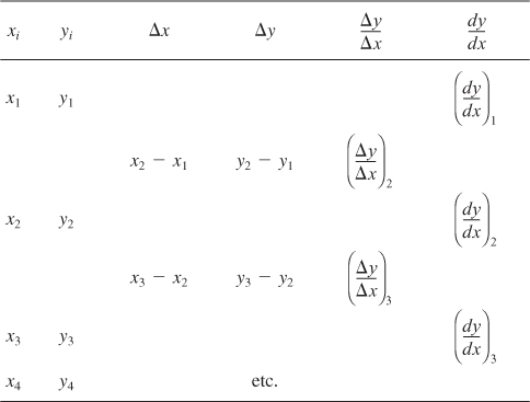
- Tabulate the (yi, xi) observations as shown in Table A-1.
- For each interval, calculate Δxn = xn – xn–1 and Δyn = yn – yn–1.
Table A-1. Graphical Differentiation
This method finds use in Chapter 5.
- Calculate Δyn / Δxn as an estimate of the average slope in an interval xn–1 to xn.
- Plot these values as a histogram versus xi. The value between x2 and x3, for example, is (y3 – y2) / (x3 – x2). Refer to Figure A.1.
Figure A.1. Equal-area differentiation.

- Next, draw in the smooth curve that best approximates the area under the histogram. That is, attempt in each interval to balance areas such as those labeled A and B, but when this approximation is not possible, balance out over several intervals (as for the areas labeled C and D). From our definitions of Δx and Δy we know that

The equal-area method attempts to estimate dy / dx so that

that is, so that the area under Δy / Δx is the same as that under dy/dx, everywhere possible.
See DVD-ROM, Appendix A, for a worked example.
- Read estimates of dy/dx from this curve at the data points x1, x2, ... and complete the table.
An example illustrating the technique is given in the DVD-ROM, Appendix A.
Differentiation is, at best, less accurate than integration. This method also clearly indicates bad data and allows for compensation of such data. Differentiation is only valid, however, when the data are presumed to differentiate smoothly, as in rate-data analysis and the interpretation of transient diffusion data.