
1.4.2 Tubular Reactor
In addition to the CSTR and batch reactors, another type of reactor commonly used in industry is the tubular reactor. It consists of a cylindrical pipe and is normally operated at steady state, as is the CSTR. Tubular reactors are used most often for gas-phase reactions. A schematic and a photograph of industrial tubular reactors are shown in Figure 1-8.
In the tubular reactor, the reactants are continually consumed as they flow down the length of the reactor. In modeling the tubular reactor, we assume that the concentration varies continuously in the axial direction through the reactor. Consequently, the reaction rate, which is a function of concentration for all but zero-order reactions, will also vary axially. For the purposes of the material presented here, we consider systems in which the flow field may be modeled by that of a plug flow profile (e.g., uniform velocity as in turbulent flow), as shown in Figure 1-9. That is, there is no radial variation in reaction rate, and the reactor is referred to as a plug-flow reactor (PFR). (The laminar flow reactor is discussed on the DVD-ROM in Chapter DVD13 and in Chapter 13 of the fourth edition of ECRE.)
Figure 1-8(a). Tubular reactor schematic. Longitudinal tubular reactor.
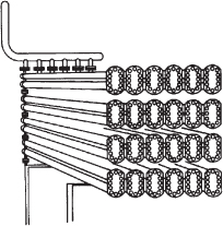
Excerpted by special permission from Chem. Eng., 63(10), 211 (Oct. 1956). Copyright 1956 by McGraw-Hill, Inc., New York, NY 10020.
Figure 1-8(b). Tubular reactor photo. Tubular reactor for production of Dimersol G.

Photo Courtesy of Editions Techniq Institut français du pétrole.
Figure 1-9. Plug-flow tubular reactor.

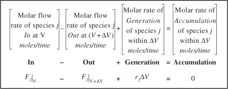
The general mole balance equation is given by Equation (1-4):
![]()
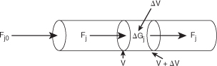
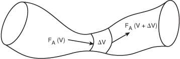
The equation we will use to design PFRs at steady state can be developed in two ways: (1) directly from Equation (1-4) by differentiating with respect to volume V, and then rearranging the result or (2) from a mole balance on species j in a differential segment of the reactor volume ΔV. Let’s choose the second way to arrive at the differential form of the PFR mole balance. The differential volume, ΔV shown in Figure 1-10, will be chosen sufficiently small such that there are no spatial variations in reaction rate within this volume. Thus the generation term, ΔGj, is
![]()
Figure 1-10. Mole balance on species j in volume ΔV.
Dividing by ΔV and rearranging
![]()
the term in brackets resembles the definition of a derivative
![]()
Taking the limit as ΔV approaches zero, we obtain the differential form of steady state mole balance on a PFR.

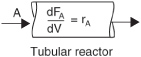
We could have made the cylindrical reactor on which we carried out our mole balance an irregular shape reactor, such as the one shown in Figure 1-11 for reactant species A.
Figure 1-11. Pablo Picasso’s reactor.
However, we see that by applying Equation (1-10), the result would yield the same equation (i.e., Equation [1-11]). For species A, the mole balance is
![]()
Consequently, we see that Equation (1-11) applies equally well to our model of tubular reactors of variable and constant cross-sectional area, although it is doubtful that one would find a reactor of the shape shown in Figure 1-11 unless it were designed by Pablo Picasso.
The conclusion drawn from the application of the design equation to Picasso’s reactor is an important one: the degree of completion of a reaction achieved in an ideal plug-flow reactor (PFR) does not depend on its shape, only on its total volume.
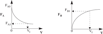
Again consider the isomerization A → B, this time in a PFR. As the reactants proceed down the reactor, A is consumed by chemical reaction and B is produced. Consequently, the molar flow rate FA decreases, while FB increases as the reactor volume V increases, as shown in Figure 1-12.
Figure 1-12. Profiles of molar flow rates in a PFR.
![]()
We now ask what is the reactor volume V1 necessary to reduce the entering molar flow rate of A from FA0 to FA1. Rearranging Equation (1-12) in the form
and integrating with limits at V = 0, then FA = FA0, and at V = V1, then FA = FA1.
![]()
V1 is the volume necessary to reduce the entering molar flow rate FA0 to some specified value FA1 and also the volume necessary to produce a molar flow rate of B of FB1.