
2.5.3 Combinations of CSTRs and PFRs in Series
The final sequences we shall consider are combinations of CSTRs and PFRs in series. An industrial example of reactors in series is shown in the photo in Figure 2-9. This sequence is used to dimerize propylene (A) into isohexanes (B), e.g.,

Figure 2-9. Dimersol G (an organometallic catalyst) unit (two CSTRs and one tubular reactor in series) to dimerize propylene into isohexanes. Institut Français du Pétrole process.

Photo courtesy of Editions Technip (Institut Français du Pétrole).
A schematic of the industrial reactor system in Figure 2-9 is shown in Figure 2-10.
Figure 2-10. Schematic of a real system.

For the sake of illustration, let’s assume that the reaction carried out in the reactors in Figure 2-10 follows the same ![]() vs. X curve given by Table 2-3.
vs. X curve given by Table 2-3.
The volumes of the first two CSTRs in series (see Example 2-5) are:
![]()
![]()
Starting with the differential form of the PFR design equation
![]()
rearranging and integrating between limits, when V = 0, then X = X2, and when V = V3, then X = X3 we obtain
![]()
The corresponding reactor volumes for each of the three reactors can be found from the shaded areas in Figure 2-11.
Figure 2-11. Levenspiel plot to determine the reactor volumes V1, V2, and V3.

The FA0/–rA curves we have been using in the previous examples are typical of those found in isothermal reaction systems. We will now consider a real reaction system that is carried out adiabatically. Isothermal reaction systems are discussed in Chapter 5 and adiabatic systems in Chapter 11.
Example 2-5. An Adiabatic Liquid-Phase Isomerization
![]()
was carried out adiabatically in the liquid phase. The data for this reversible reaction are given in Table E2-5.1. (Example 11.3 shows how the data in Table E2-5.1 were generated.)

Don’t worry how we got this data or why the (1/–rA) looks the way it does; we will see how to construct this table in Chapter 11. It is real data for a real reaction carried out adiabatically, and the reactor scheme shown below in Figure E2-5.1 is used.
Figure E2-5.1. Reactors in series.
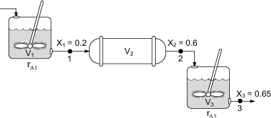
Calculate the volume of each of the reactors for an entering molar flow rate of n-butane of 50 kmol/hr.
Taking the reciprocal of –rA and multiplying by FA0, we obtain Table E2-5.2.
![]()
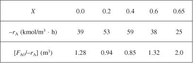
when X = 0.2, then ![]()
E2-5.1
![]()
E2-5.2
![]()
b. For the PFR,
![]()
Using Simpson’s three-point formula with ΔX = (0.6 – 0.2)/2 = 0.2, and X1 = 0.2, X2 = 0.4, and X3 = 0.6.
E2-5.3

E2-5.4
![]()
c. For the last reactor and the second CSTR, mole balance on A for the CSTR:
In – Out + Generation = 0
E2-5.5
![]()
Rearranging

Simplifying
![]()
We find from Table E2-5.2 that at X3 = 0.65, then ![]()
V3 = 2 m3 (0.65 – 0.6) = 0.1 m3
![]()
A Levenspiel plot of (FA0/–rA) vs. X is shown in Figure E2-5.2.
Figure E2-5.2. Levenspiel plot for adiabatic reactors in series.

For this adiabatic reaction the three reactors in series resulted in an overall conversion of 65%. The maximum conversion we can achieve is the equilibrium conversion which is 68% and is shown by the dashed line in Figure E2-5.2. Recall that at equilibrium, the rate of reaction is zero and an infinite reactor volume is required to reach equilibrium ![]()
Analysis: For exothermic reactions that are not carried out isothermally, the rate usually increases at the start of the reaction because reaction temperature increases. However, as the reaction proceeds the rate eventually decreases as the conversion increases as the reactants are consumed. These two competing effects give the bowed shape of the curve in Figure (E2-5.2) which will be discussed in detail in Chapter 12. Under these circumstances, we saw that a CSTR will require a smaller volume than a PFR at low conversions.