Chapter 5. Isothermal Reactor Design: Conversion

5.1 Design Structure for Isothermal Reactors

One of the primary goals of this chapter is to solve chemical reaction engineering (CRE) problems by using logic rather than memorizing which equation applies where. It is the author’s experience that following this structure, shown in Figure 5-1, will lead to a greater understanding of isothermal reactor design. We begin by applying our general mole balance equation (level ) to a specific reactor to arrive at the design equation for that reactor (level ). If the feed conditions are specified (e.g., N_A0 or F_A0), all that is required to evaluate the design equation is the rate of reaction as a function of conversion at the same conditions as those at which the reactor is to be operated (e.g., temperature and pressure). When –r_A = f(X) is known or given, one can go directly from level to the last level, level , to determine either the batch time or reactor volume necessary to achieve the specified conversion.

Figure 5-1. Isothermal reaction design algorithm for conversion.

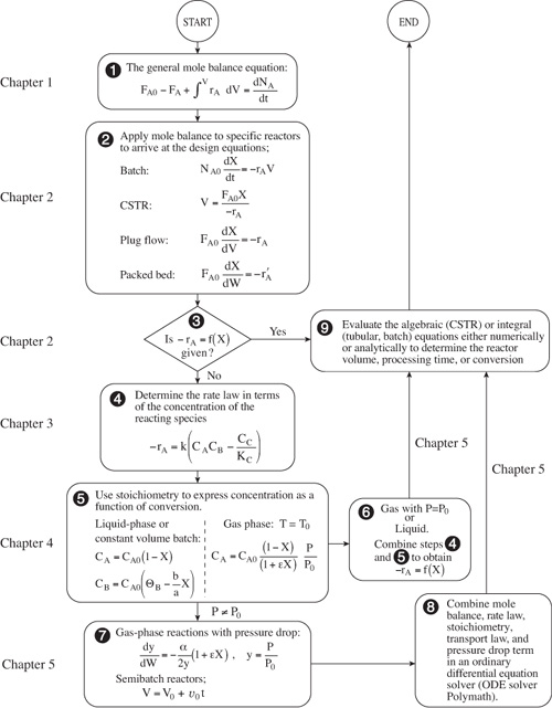
When the rate of reaction is not given explicitly as a function of conversion, we must proceed to level , where the rate law must be determined by either finding it in books or journals or by determining it experimentally in the laboratory. Techniques for obtaining and analyzing rate data to determine the reaction order and rate constant are presented in Chapter 7. After the rate law has been established, one has only to use stoichiometry (level ) together with the conditions of the system (e.g., constant volume, temperature) to express concentration as a function of conversion.

For liquid-phase reactions and for gas-phase reactions with no pressure drop (P = P₀), one can combine the information in levels and , to express the rate of reaction as a function of conversion and arrive at level . It is now possible to determine either the time or reactor volume necessary to achieve the desired conversion by substituting the relationship linking conversion and rate of reaction into the appropriate design equation (level ).

For gas-phase reactions in packed beds where there is a pressure drop, we need to proceed to level to evaluate the pressure ratio (P / P₀) in the concentration term using the Ergun equation (Section 5.5). In level , we combine the equations for pressure drop in level with the information in levels and , to proceed to level , where the equations are then evaluated in the appropriate manner (i.e., analytically using a table of integrals, or numerically using an ODE solver). Although this structure emphasizes the determination of a reaction time or reactor volume for a specified conversion, it can also readily be used for other types of reactor calculations, such as determining the conversion for a specified volume. Different manipulations can be performed in level to answer the different types of questions mentioned here.

The structure shown in Figure 5-1 allows one to develop a few basic concepts and then to arrange the parameters (equations) associated with each concept in a variety of ways. Without such a structure, one is faced with the possibility of choosing or perhaps memorizing the correct equation from a multitude of equations that can arise for a variety of different combinations of reactions, reactors, and sets of conditions. The challenge is to put everything together in an orderly and logical fashion so that we can arrive at the correct equation for a given situation.

Fortunately, by using the algorithm to formulate CRE problems shown in Figure 5-2, which happens to be analogous to the algorithm for ordering dinner from a fixed-price menu in a fine French restaurant, we can eliminate virtually all memorization. In both of these algorithms, we must make choices in each category. For example, in ordering from a French menu, we begin by choosing one dish from the appetizers listed. Step 1 of the CRE algorithm shown in Figure 5-2 is to begin by choosing the appropriate mole balance for one of the three types of reactors shown. In Step 2 we choose the rate law (entrée), and in Step 3 we specify whether the reaction is gas or liquid phase (cheese or dessert). Finally, in Step 4 we combine Steps 1, 2, and 3 and either obtain an analytical solution or solve the equations using an ODE solver. (See the complete French menu on the DVD-ROM Chapter 5 Summary Notes).

Figure 5-2. Algorithm for isothermal reactors.

We now will apply this algorithm to a specific situation. Suppose that we have, as shown in Figure 5-2, mole balances for three reactors, three rate laws, and the equations for concentrations for both liquid and gas phases. In Figure 5-2 we see how the algorithm is used to formulate the equation to calculate the PFR reactor volume for a first-order gas-phase reaction. The pathway to arrive at this equation is shown by the ovals connected to the dark lines through the algorithm. The dashed lines and the boxes represent other pathways for solutions to other situations. The algorithm for the pathway shown is

1. Mole balances, choose species A reacting in a PFR
2. Rate laws, choose the irreversible first-order reaction
3. Stoichiometry, choose the gas-phase concentration
4. Combine steps 1, 2, and 3 to arrive at Equation A
5. Evaluate. The combine step can be evaluated either
   

   a. Analytically (Appendix Al)

   b. Graphically (Chapter 2)

   c. Numerically (Appendix A4)

In Figure 5-2 we chose to integrate Equation A for constant temperature and pressure to find the volume necessary to achieve a specified conversion (or calculate the conversion that can be achieved in a specified reactor volume). Unless the parameter values are zero, we typically don’t substitute numerical values for parameters in the combine step until the very end.

For the case of isothermal operation with no pressure drop, we were able to obtain an analytical solution, given by equation B, which gives the reactor volume necessary to achieve a conversion X for a first-order gas-phase reaction carried out isothermally in a PFR. However, in the majority of situations, analytical solutions to the ordinary differential equations appearing in the combine step are not possible. Consequently, we include Polymath, or some other ODE solver such as MATLAB, in our menu in that it makes obtaining solutions to the differential equations much more palatable.

5.2 Batch Reactors (BRs)

One of the jobs in which chemical engineers are involved is the scale-up of laboratory experiments to pilot-plant operation or to full-scale production. In the past, a pilot plant would be designed based on laboratory data. In this section we show how to analyze a laboratory-scale batch reactor in which a liquid-phase reaction of known order is being carried out.

In modeling a batch reactor, we assume there is no inflow or outflow of material and that the reactor is well mixed. For most liquid-phase reactions, the density change with reaction is usually small and can be neglected (i.e., V = V₀). In addition, for gas-phase reactions in which the batch reactor volume remains constant, we also have V = V₀.