
7.4.2 Finding the Rate Law Parameters
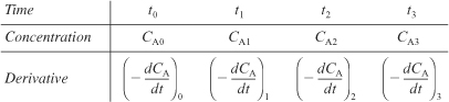
Now, using either the graphical method, differentiation formulas, or the polynomial derivative, the following table can be set up:
The reaction order can now be found from a plot of ln (–dCA/dt) as a function of ln CA, as shown in Figure 7-5(a), since

Before solving an example problem, review the steps to determine the reaction rate law from a set of data points (Table 7-1).
Example 7-2. Determining the Rate Law
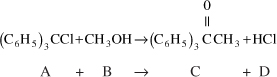
The reaction of triphenyl methyl chloride (trityl) (A) and methanol (B) discussed in Example 7-1 is now analyzed using the differential method.
The concentration-time data in Table E7-2.1 was obtained in a batch reactor
The initial concentration of methanol was 0.5 mol/dm3.
Part (1) Determine the reaction order with respect to triphenyl methyl chloride.
Part (2) In a separate set of experiments, the reaction order wrt methanol was found to be first order. Determine the specific reaction rate constant.
Part (1) Find reaction order with respect to trityl.
- Postulate a rate law.

- Process your data in terms of the measured variable, which in this case is CA.
- Look for simplifications. Because the concentration of methanol is 10 times the initial concentration of triphenyl methyl chloride, its concentration is essentially constant

Substituting for CB in Equation (E7-2.1)

- Apply the CRE algorithm.
Mole Balance


Stoichiometry: Liquid V = V0

Combine: Mole balance, rate law, and stoichiometry


Evaluate: Taking the natural log of both sides of Equation (E7-2.5)
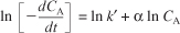
The slope of a plot of ln
 versus ln CA will yield the reaction order α with respect to triphenyl methyl chloride (A).
 - Find as a function of CA from concentration-time data.
- 5A.1a Graphical Method. We now construct Table E7-2.2.
The derivative (–dCA/dt) is determined by calculating and plotting (–ΔCA/Δt) as a function of time, t, and then using the equal-area differentiation technique (Appendix A.2) to determine (–dCA/dt) as a function of CA. First, we calculate the ratio (–ΔCA/Δt) from the first two columns of Table E7-2.2; the result is written in the third column.

Next we use Table E7-2.2 to plot the third column as a function of the first column in Figure E7-1.1 [i.e., (–ΔCA/Δt) versus t]. Using equal-area differentiation, the value of (–dCA/dt) is read off the figure (represented by the arrows); then it is used to complete the fourth column of Table E7-2.2.
Figure E7-2.1. Graphical differentiation.

The results to find (–dCA/dt) at each time, t, and concentration, CA, are summarized in Table E7-2.3.
We will now use Table E7-2.3 to plot column ![]() as a function of column 3 (CA × 1,000) on log-log paper as shown in Figure E7-2.2. We could also substitute the parameter values in Table E7-2.3 into Excel to find α and k′. Note that most of the points for all methods fall virtually on top of one another.
as a function of column 3 (CA × 1,000) on log-log paper as shown in Figure E7-2.2. We could also substitute the parameter values in Table E7-2.3 into Excel to find α and k′. Note that most of the points for all methods fall virtually on top of one another.
Table E7-2.3. Summary of Processed Data
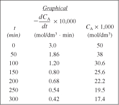
Figure E7-2.2. Excel plot to determine α and k.
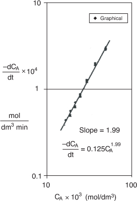
From Figure E7-2.2, we found the slope to be 1.99, so that the reaction is said to be second order (α = 2.0) with respect to triphenyl methyl chloride. To evaluate k′, we can evaluate the derivative in Figure E7-2.2 at CAp = 20 × 10–3 mol/dm3, which is
![]()
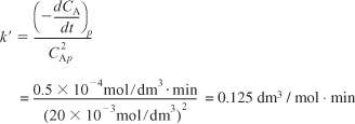
As will be shown in Section 7-5, we could also use nonlinear regression on Equation (E7-1.5) to find k′:
![]()
The Excel graph shown in Figure E7-2.2 gives α = 1.99 and k′ = 0.13 dm3/mol · min. We could set α = 2 and regress again to find k′ = 0.122 dm3/mol · min.

ODE Regression. There are techniques and software becoming available whereby an ODE solver can be combined with a regression program to solve differential equations, such as
![]()
to find kA and α from concentration–time data.
Part (2) The reaction was said to be first order with respect to methanol, β = 1,
![]()
Assuming CB0 is constant at 0.5 mol/dm3 and solving for k yields1

The rate law is
![]()
Analysis: In this example the differential method of data analysis was used to find the reaction order with respect to trityl (α = 1.99) and the pseudo rate constant (k′ = 0.125 (dm3/mol)/min). The reaction order was rounded up to α = 2 and the data was regressed again to obtain k′ = 0.122 (dm3/mol)/min, again knowing k′ and CB0 and the true rate constant is k = 0.244 (dm3/mol)2/min.
By comparing the methods of analysis of the rate data presented in Examples 7-1 and 7-2, we note that the differential method tends to accentuate the uncertainties in the data, while the integral method tends to smooth the data, thereby disguising the uncertainties in it. In most analyses, it is imperative that the engineer know the limits and uncertainties in the data. This prior knowledge is necessary to provide for a safety factor when scaling up a process from laboratory experiments to design either a pilot plant or full-scale industrial plant.
7.5 Nonlinear Regression
In nonlinear regression analysis, we search for those parameter values that minimize the sum of the squares of the differences between the measured values and the calculated values for all the data points. Not only can nonlinear regression find the best estimates of parameter values, it can also be used to discriminate between different rate law models, such as the Langmuir–Hinshelwood models discussed in Chapter 10. Many software programs are available to find these parameter values so that all one has to do is enter the data. The Polymath software will be used to illustrate this technique. In order to carry out the search efficiently, in some cases one has to enter initial estimates of the parameter values close to the actual values. These estimates can be obtained using the linear-least-squares technique discussed on the DVD-ROM Professional Reference Shelf R7.3.
We will now apply nonlinear regression to reaction rate data to determine the rate law parameters. Here we make initial estimates of the parameter values (e.g., reaction order, specific rate constant) in order to calculate the concentration for each data point, Cic, obtained by solving an integrated form of the combined mole balance and rate law. We then compare the measured concentration at that point, Cim, with the calculated value, Cic, for the parameter values chosen. We make this comparison by calculating the sum of the squares of the differences at each point Σ(Cim – Cic)2. We then continue to choose new parameter values and search for those values of the rate law that will minimize the sum of the squared differences of the measured concentrations, Cim, and the calculated concentrations values, Cic. That is, we want to find the rate law parameters for which the sum of all data points Σ(Cim – Cic)2 is a minimum. If we carried out N experiments, we would want to find the parameter values (e.g., E, activation energy, reaction orders) that minimize the quantity
![]()
where
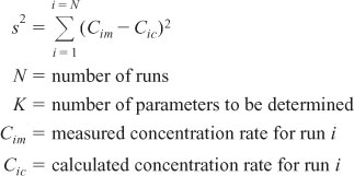
One notes that if we minimize s2 we minimize σ2.
To illustrate this technique, let’s consider the reaction
![]()
for which we want to learn the reaction order, α, and the specific reaction rate, k,
![]()
The reaction rate will be measured at a number of different concentrations. We now choose values of k and α and calculate the rate of reaction (Cic) at each concentration at which an experimental point was taken. We then subtract the calculated value (Cic) from the measured value (Cim), square the result, and sum the squares for all the runs for the values of k and α that we have chosen.
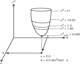
This procedure is continued by further varying α and k until we find those values of k and α that minimize the sum of the squares. Many well-known searching techniques are available to obtain the minimum value ![]() .2 Figure 7-7 shows a hypothetical plot of the sum of the squares as a function of the parameters α and k:
.2 Figure 7-7 shows a hypothetical plot of the sum of the squares as a function of the parameters α and k:
![]()
Look at the top circle. We see that there are many combinations of α and k (e.g., α = 2.2, k = 4.8 or α = 1.8, k = 5.3) that will give a value of σ2 = 57. The same is true for σ2 = 1.85. We need to find the combination of α and k that gives the lowest value of σ2.
In searching to find the parameter values that give the minimum of the sum of squares σ2, one can use a number of optimization techniques or soft ware packages. The searching procedure begins by guessing parameter values and then calculating Cc and then σ2 for these values. Next, a few sets of parameters are chosen around the initial guess, and σ2 is calculated for these sets as well. The search technique looks for the smallest value of σ2 in the vicinity of the initial guess and then proceeds along a trajectory in the direction of decreasing σ2 to choose different parameter values and determine the corresponding σ2. The trajectory is continually adjusted so as to always proceed in the direction of decreasing σ2 until the minimum value of σ2 is reached. For example, in Figure 7-6 the search technique keeps choosing combinations of α and k until a minimum value of σ2 = 0.045 (mol/dm3)2 is reached. The combination that gives that minimum is α = 2 and k = 5.0 dm3/mol·min. If the equations are highly non-linear, the initial guesses of α and k are very important.

Figure 7-6. Minimum sum of squares.
A number of software packages are available to carry out the procedure to determine the best estimates of the parameter values and the corresponding confidence limits. All one has to do is to type the experimental values in the computer, specify the model, enter the initial guesses of the parameters, and then push the “compute” button, and the best estimates of the parameter values along with 95% confidence limits appear. If the confidence limits for a given parameter are larger than the parameter itself, the parameter is probably not significant and should be dropped from the model. After the appropriate model parameters are eliminated, the software is run again to determine the best fit with the new model equation.