
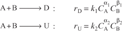
8.3.3 Reactor Selection and Operating Conditions
Next, consider two simultaneous reactions in which two reactants, A and B, are being consumed to produce a desired product, D, and an unwanted product, U, resulting from a side reaction. The rate laws for the reactions

are
![]()
![]()
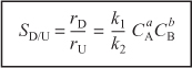
The instantaneous selectivity
![]()
is to be maximized. Shown in Figure 8-2 are various reactor schemes and conditions that might be used to maximize SD/U.
Figure 8-2. Different reactors and schemes for minimizing the unwanted product.

The two reactors with recycle shown in (i) and (j) can be used for highly exothermic reactions. Here the recycle stream is cooled and returned to the reactor to dilute and cool the inlet stream, thereby avoiding hot spots and runaway reactions. The PFR with recycle is used for gas-phase reactions, and the CSTR is used for liquid-phase reactions. The last two reactors, (k) and (l), are used for thermodynamically limited reactions where the equilibrium lies far to the left (reactant side)
![]()
and one of the products must be removed (e.g., C) for the reaction to continue to completion. The membrane reactor (k) is used for thermodynamically limited gas-phase reactions, while reactive distillation (l) is used for liquid-phase reactions when one of the products has a higher volatility (e.g., C) than the other species in the reactor.
In making our selection of a reactor, the criteria are safety, selectivity, yield, temperature control, and cost.
Example 8-2. Choice of Reactor and Conditions to Minimize Unwanted Products
consider all possible combinations of reaction orders and select the reaction scheme that will maximize SD/U.
Case I: α1>α2, β1>β2. Let a = α1 – α2 and b = β1 – β2, where a and b are positive constants. Using these definitions, we can write Equation (8-16) in the form
To maximize the ratio rD/rU, maintain the concentrations of both A and B as high as possible. To do this, use
• A tubular reactor [Figure 8-2(b)]
• A batch reactor [Figure 8-2(c)]
• High pressures (if gas phase), and reduce inerts
Case II: α1>α2, β1<β2. Let a = α1 – α2 and b = β2 – β1, where a and b are positive constants. Using these definitions, we can write Equation (8-16) in the form
![]()
To make SD/U as large as possible, we want to make the concentration of A high and the concentration of B low. To achieve this result, use
• A semibatch reactor in which B is fed slowly into a large amount of A [Figure 8-2(d)]
• A membrane reactor or a tubular reactor with side streams of B continually fed to the reactor [Figure 8-2(f)]
• A series of small CSTRs with A fed only to the first reactor and small amounts of B fed to each reactor. In this way B is mostly consumed before the CSTR exit stream flows into the next reactor [Figure 8-2(h)]
Case III: α1<α2, β1<β2. Let a = α2 – α1 and b = β2 – β1, where a and b are positive constants. Using these definitions, we can write Equation (8-16) in the form
![]()
To make SD/U as large as possible, the reaction should be carried out at low concentrations of A and of B. Use
• A CSTR [Figure 8-2(a)]
• A tubular reactor in which there is a large recycle ratio [Figure 8-2(i)]
• A feed diluted with inerts
• Low pressure (if gas phase)
Case IV: α1<α2, β1>β2. Let a = α2 – α1 and b = β1 – β2, where a and b are positive constants. Using these definitions, we can write Equation (8-16) in the form

To maximize SD/U, run the reaction at high concentrations of B and low concentrations of A. Use
• A semibatch reactor with A slowly fed to a large amount of B [Figure 8-2(e)]
• A membrane reactor or a tubular reactor with side streams of A [Figure 8-2(g)]
• A series of small CSTRs with fresh A fed to each reactor
Analysis: In this very important example we showed how to use the instantaneous selectivity, SD/U, to guide the selection of the type of reactor and reactor system to maximize the selectivity with respect to the desired species D.
8.4 Reactions in Series
In Section 8.1, we saw that the undesired product could be minimized by adjusting the reaction conditions (e.g., concentration, temperature) and by choosing the proper reactor. For series (i.e., consecutive) reactions, the most important variable is time: space-time for a flow reactor and real-time for a batch reactor. To illustrate the importance of the time factor, we consider the sequence
![]()

in which species B is the desired product.
If the first reaction is slow and the second reaction is fast, it will be extremely difficult to produce species B. If the first reaction (formation of B) is fast and the reaction to form C is slow, a large yield of B can be achieved. However, if the reaction is allowed to proceed for a long time in a batch reactor, or if the tubular flow reactor is too long, the desired product B will be converted to the undesired product C. In no other type of reaction is exactness in the calculation of the time needed to carry out the reaction more important than in series reactions.
Example 8-3. Series Reactions in a Batch Reactor
The elementary liquid phase series reaction
![]()
is carried out in a batch reactor. The reaction is heated very rapidly to the reaction temperature where it is held at this temperature until the time it is quenched.
a. Plot and analyze the concentrations of species A, B, and C as a function of time.
b. Calculate the time to quench the reaction when the concentration of B will be a maximum.
c. What are the overall selectivity and yields at this quench time?
CA0 = 2M, k1 = 0.5h–1, k2 = 0.2h–1
Part (a)
Number the reactions:
The preceding series reaction can be written as two reactions
(1) Reaction 1 ![]() –r1A = k1CA
–r1A = k1CA
(2) Reaction 2 ![]() –r2B = k2CB
–r2B = k2CB
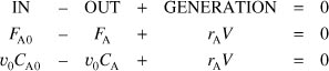
1. Mole Balances:
2A.Mole Balance on A:
![]()
a. Mole Balance in terms of concentration for V = V0 becomes
E8-3.1
![]()
b. Rate law for Reaction 1: Reaction is elementary
E8-3.2
![]()
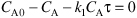
c. Combining the mole balance and rate law
E8-3.3
![]()
Integrating with the initial condition CA = CA0 at t = 0
E8-3.4
![]()
Solving for CA
E8-3.5
![]()

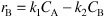
2B. Mole Balance on B:
a. Mole Balance for a constant volume batch reactor
E8-3.6
![]()
b. Rates:
Rate Laws
Elementary reactions
E8-3.7
![]()
Relative Rates
Rate of formation of B in Reaction 1 equals the rate of disappearance of A in Reaction 1
E8-3.8
![]()
The net rate of reaction of B will be the rate of formation of B in reaction (1) plus the rate of formation of B in reaction (2)
E8-3.9
![]()
E8-3.10
![]()
c. Combining the mole balance and rate law
E8-3.11
![]()
Rearranging and substituting for CA
E8-3.12
![]()
Using the integrating factor gives
E8-3.13
![]()
There is a tutorial on the integrating factor in Appendix A and on the Web.
At time t = 0, CB = 0. Solving Equation (E8-3.13) gives
E8-3.14
2C. Mole Balance on C:
The mole balance on C is similar to Equation (E8-3.1)
![]()
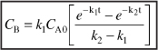
The rate of formation of C is just the rate of disappearance of B in reaction (2), i.e., rC = –r2B = k2CB
![]()
Substituting for CB
![]()
and integrating with CC = 0 at t = 0 gives
![]()
Note that as t → ∞ then CC = CA0 as expected. We also note the concentration of C, CC, could have been obtained more easily from an overall balance.
![]()
The concentration of A, B, and C are shown as a function of time below
Figure E8-3.1. Concentration trajectories in a batch reactor.

Part (b)
4. Optimum Yield
We note from Figure E8-3.1 that the concentration of B goes through a maximum. Consequently, to find the maximum we need to differentiate Equation E8-3.14 and set it to zero.
![]()
Solving for tmax gives
![]()
Substituting Equation (E8-3.20) into Equation (E8-3.5), we find the concentration of A at the maximum for CB is
![]()

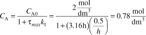
Similarly, the concentration of B at the maximum is
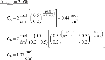
5. Evaluate: For CA0 = 2 mol/dm3, k1 = 0.5h–1, and k2 = 0.2h–1 the concentrations as a function of time are:
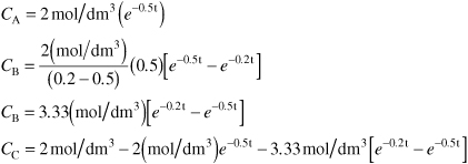
Substituting in Equation (E8-3.20)

The time to quench the reaction is at 3.05h.
The concentration of C at the time we quench the reaction is
CC = CA0 – CA – CB = 2 – 0.44 – 1.07 = 0.49 mol/dm3
Part (c)
The selectivity is
![]()
The yield is
![]()
Analysis: In this example we applied our CRE algorithm for multiple reactions to the series reaction A → B → C. Here we obtained an analytical solution to find the time at which the concentration of the desired product B was a maximum and, consequently, the time to quench the reaction. We also calculated the concentrations of A, B, and C at this time, along with the selectivity and yield.
We will now carry out this same series reaction in a CSTR.
Example 8-4. Series Reaction in a CSTR
The reactions discussed in Example 8-3 are now to be carried out in a CSTR.
![]()
a. Determine the exit concentrations from the CSTR.
b. Find the value of the space time τ that will maximize the concentration of B.
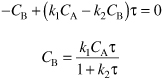
Part (a)
-
a. Mole Balance on A:
Dividing by υ0, rearranging and recalling that τ = V/υ0, we obtain
E8-4.1

b. Rates
The laws and net rates are the same as in Example 8-3.
E8-4.2

c. Combining the mole balance of A with the rate of disappearance of A
E8-4.3
Solving for CA
E8-4.4

We now use the same algorithm for Species B we did for Species A to solve for the concentration of B
-
a. Mole Balance on B:

Dividing by υ0 and rearranging
E8-4.5

b. Rates
The laws and net rates are the same as in Example 8-3.
Net Rates
E8-4.6
c. Combine
E8-4.7
Substituting for CA
E8-4.8
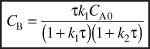
- Mole Balance on C:

Rates
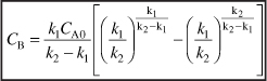
Part (b) Optimum Concentration of B
To find the maximum concentration of B, we set the differential of Equation (E8-4.8) with respect to τ equal to zero
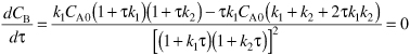
Solving for t at which the concentration of B is a maximum at

The exiting concentration of B at the optimum value of τ is
![]()
Substituting Equation (E8-4.11) for τmax in Equation (E8-4.12)
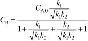
Rearranging we find the concentration of B at the optimum space time is
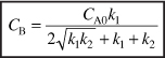
Evaluation
![]()
At τmax

The conversion is
![]()
The selectivity is
![]()
The yield is
![]()
Analysis: The CRE algorithm for multiple reactions was applied to the series reaction A → B → C in a CSTR to find the CSTR space time necessary to maximize the concentration of B, i.e., τ = 3.16h. The conversion at this space time is 61%, the selectivity, ![]() , is 1.60 and the yield,
, is 1.60 and the yield, ![]() , is 0.63. The conversion and selectivity are less for the CSTR than those for the batch reactor at the time of quenching.
, is 0.63. The conversion and selectivity are less for the CSTR than those for the batch reactor at the time of quenching.
If the series reaction were carried out in a PFR, the results would essentially be those of a batch reactor where we replaced the time variable “t” with the space time, “τ”. Data for the series reaction
![]()
is compared for different values of the specific reaction rates, k1 and k2, in Figure 8-3.
Figure 8-3. Yield of acetaldehyde as a function of ethanol conversion. Data were obtained at 518 K. Data points (in order of increasing ethanol conversion) were obtained at space velocities of 26,000, 52,000, 104,000, and 208,000 h–1. The curves were calculated for a first-order series reaction in a plug-flow reactor and show yield of the intermediate species B as a function of the conversion of reactant for various ratios of rate constants k2 and k1.

A complete analysis of this reaction carried out in a PFR is given on the DVD-ROM.
Many metabolic reactions involve a large number of sequential reactions, such as those that occur in the coagulation of blood.
Cut → Blood → Clotting
Blood coagulation is part of an important host defense mechanism called hemostasis, which causes the cessation of blood loss from a damaged vessel. The clotting process is initiated when a non-enzymatic lipoprotein (called the tissue factor) contacts blood plasma because of cell damage. The tissue factor (TF), is normally not in contact with plasma (see Figure B) because of an intact endothelium. The rupture (e.g., cut) of the endothelium exposes the plasma to TF and a cascade of series reactions proceeds (Figure C). These series reactions ultimately result in the conversion of fibrinogen (soluble) to fibrin (insoluble), which produces the clot. Later, as wound healing occurs, mechanisms that restrict formation of fibrin clots, necessary to maintain the fluidity of the blood, start working.
Figure A. Normal clot coagulation of blood.
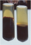
Picture courtesy of: Dietrich Mebs, Venomous and Poisonous Animals, Stuttgart: Medpharm, (2002), p. 305.
Figure B. Schematic of separation of TF (A) and plasma (B) before cut occurs.
Figure C. Cut allows contact of plasma to initiate coagulation. (A + B → Cascade)
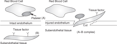
*Platelets provide procoagulant phospholipids-equivalent surfaces upon which the complex-dependent reactions of the blood coagulation cascade are localized.

An abbreviated form (1) of the initiation and following cascade metabolic reactions that can capture the clotting process is
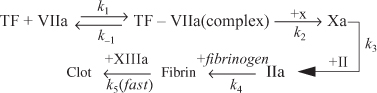
In order to maintain the fluidity of the blood, the clotting sequence (2) must be moderated. The reactions that attenuate the clotting process are

where TF = tissue factor, VIIa = factor novoseven, X = Stuart Prower factor, Xa = Stuart Prower factor activated, II = prothrombin, IIa = thrombin, ATIII = antithrombin, and XIIIa = factor XIIIa.
Symbolically, the clotting equations can be written as
Cut → A + B → C → D → E → F → Clot
One can model the clotting process in a manner identical to the series reactions by writing a mole balance and rate law for each species, such as

and then using Polymath to solve the coupled equations to predict the thrombin (shown in Figure D) and other species concentration as a function of time as well as to determine the clotting time. Laboratory data are also shown below for a TF concentration of 5 pM. One notes that when the complete set of equations is used, the Polymath output is identical to Figure E. The complete set of equations, along with the Polymath Living Example Problem code, is given in the Solved Problems on the DVD-ROM. You can load the program directly and vary some of the parameters.
Figure D. Total thrombin as a function of time with an initiating TF concentration of 25 pM (after running Polymath) for the abbreviated blood clotting cascade.

Figure E. Total thrombin as a function of time with an initiating TF concentration of 25 pM. Full blood clotting cascade.

Figure courtesy of M. F. Hockin et al., “A Model for the Stoichiometric Regulation of Blood Coagulation,” The Journal of Biological Chemistry, 277[21], pp. 18322–18333 2002. Copyright © 2002, by the American Society for Biochemistry and Molecular Biology.

8.5 Complex Reactions
A complex reaction system consists of a combination of interacting series and parallel reactions. An overview of this algorithm is very similar to the one given in Chapter 6 for writing the mole balances in terms of molar flow rates and concentrations (i.e., Figure 6-1). After numbering each reaction, we write a mole balance on each species, similar to those in Figure 6-1. The major difference between the two algorithms is in the rate law step. As shown in Table 8-2, we have three steps (3, 4 and 5) to find the net rate of reaction for each species in terms of the concentration of the reacting species. As an example we shall study the following complex reactions
![]()
carried out in a PBR, a CSTR, and a semibatch reactor.