9.3.1 Competitive Inhibition

Competitive inhibition is of particular importance in pharmacokinetics (drug therapy). If a patient were administered two or more drugs that react simultaneously within the body with a common enzyme, cofactor, or active species, this interaction could lead to competitive inhibition in the formation of the respective metabolites and produce serious consequences.

In competitive inhibition, another substance, I, competes with the substrate for the enzyme molecules to form an inhibitor–enzyme complex, as shown in Figure 9-9.

Figure 9-9. Steps in competitive enzyme inhibition.

(a) Competitive inhibition. Courtesy of D. L. Nelson and M. M. Cox, Lehninger Principles of Biochemistry, 3rd ed. (New York: Worth Publishers, 2000), p. 266.

In addition to the three Michaelis–Menten reaction steps, there are two additional steps as the inhibitor reversely ties up the enzyme, as shown in reaction steps 4 and 5.

The rate law for the formation of product is the same [cf. Equations (9-18A) and (9-19)] as it was before in the absence of inhibitor

9-34

Applying the PSSH, the net rate of reaction of the enzyme–substrate complex is

9-35

The net rate of formation of inhibitor-substrate complex is also zero

9-36

The total enzyme concentration is the sum of the bound and unbound enzyme concentrations

9-37

Combining Equations (9-35), (9-36), and (9-37) and solving for (E · S) and substituting in Equation (9-34) and simplifying

9-38

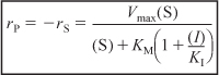
V_max and K_M are the same as before when no inhibitor is present, that is,

and the inhibition constant K_I (mol/dm³) is

By letting , we can see that the effect of adding a competitive inhibitor is to increase the “apparent” Michaelis constant, . A consequence of the larger “apparent” Michaelis constant K_M is that a larger substrate concentration is needed for the rate of substrate decomposition, –r_S, to reach half its maximum rate.

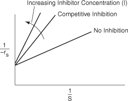
Rearranging Equation (9-38) in order to generate a Lineweaver–Burk plot,

9-39

From the Lineweaver–Burk plot (Figure 9-10), we see that as the inhibitor (I) concentration is increased, the slope increases (i.e., the rate decreases), while the intercept remains fixed.

Figure 9-10. Lineweaver–Burk plot for competitive inhibition.