Chapter 1. Scope and Language of Thermodynamics

Chemical processes involve streams undergoing various transformations. One example is shown in Figure 1-1: raw materials are fed into a heated reactor, where they react to form products. The effluent stream, in this case a liquid, contains the products of the reaction, any unreacted raw materials, and possibly other by-products. This stream is pumped out of the reactor into a heat exchanger, where it partially boils. The vapor/liquid mixture is fed into a tank, which collects the vapor at the top, and liquid at the bottom. The streams that exit this tank are finally cooled down and sent to the next stage of the process. Actual processes are generally more complex and may involve many streams and several interconnected units. Nonetheless, the example in Figure 1-1 contains all the basic ingredients likely to be found in any chemical plant: heating, cooling, pumping, reactions, phase transformations.

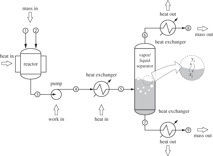
Figure 1-1: Typical chemical process.

It is the job of the chemical engineer to compute the material and energy balances around such process: This includes the flow rates and compositions of all streams, the power requirements of pumps, compressors and turbines, and the heat loads in the heat exchangers. The chemical engineer must also determine the conditions of pressure and temperature that are required to produce the desired effect, whether this is a chemical reaction or a phase transformation. All of this requires the knowledge of various physical properties of a mixture: density, heat capacity, boiling temperature, heat of vaporization, and the like. More specifically, these properties must be known as a function of temperature, pressure, and composition, all of which vary from stream to stream. Energy balances and property estimation may appear to be separate problems, but they are not: both calculations require the application of the same fundamental principles of thermodynamics.

The name thermodynamics derives from the Greek thermotis (heat) and dynamiki (potential, power). Its historical roots are found in the quest to develop heat engines, devices that use heat to produce mechanical work. This quest, which was instrumental in powering the industrial revolution, gave birth to thermodynamics as a discipline that studies the relationship between heat, work, and energy. The elucidation of this relationship is one of the early triumphs of thermodynamics and a reason why, even today, thermodynamics is often described as the study of energy conversions involving heat. Modern thermodynamics is a much broader discipline whose focus is the equilibrium state of systems composed of very large numbers of molecules. Temperature, pressure, heat, and mechanical work, as manifested through the expansion and compression of matter, are understood to arise from interactions at the molecular level. Heat and mechanical work retain their importance but the scope of the modern discipline is far wider than its early developers would have imagined, and encompasses many different systems containing huge numbers of “particles,” whether these are molecules, electron spins, stars, or bytes of digital information. The term chemical thermodynamics refers to applications to molecular systems. Among the many scientists who contributed to the development of modern thermodynamics, J. Willard Gibbs stands out as one whose work revolutionized the discipline by providing the tools to connect the macroscopic properties of thermodynamics to the microscopic properties of molecules. His name is now associated with the Gibbs free energy, a thermodynamic property of fundamental importance in phase and chemical equilibrium.

Figure 1-2: J. W. Gibbs.

Chemical engineering thermodynamics is the subset that applies thermodynamics to processes of interest to chemical engineers. One important task is the calculation of energy requirements of a process and, more broadly, the analysis of energy utilization and efficiency in chemical processing. This general problem is discussed in the first part of the book, Chapters 2 through 7. Another important application of chemical engineering thermodynamics is in the design of separation units. The vapor-liquid separator in Figure 1-1 does more than just separate the liquid portion of the stream from the vapor. When a multicomponent liquid boils, the more volatile (“lighter”) components collect preferentially in the vapor and the less volatile (“heavier”) ones remain mostly in the liquid. This leads to partial separation of the initial mixture. By staging multiple such units together, one can accomplish separations of components with as high purity as desired. The determination of the equilibrium composition of two phases in contact with each other is an important goal of chemical engineering thermodynamics. This problem is treated in the second part of the book and the first part is devoted to the behavior of single-component fluids. Overall then, the chemical engineer uses thermodynamics to

1. Perform energy and material balances in unit operations with chemical reactions, separations, and fluid transformations (heating/cooling, compression/ expansion),

2. Determine the various physical properties that are required for the calculation of these balances,

3. Determine the conditions of equilibrium (pressure, temperature, composition) in phase transformations and chemical reactions.

These tasks are important for the design of chemical processes and for their proper control and troubleshooting. The overall learning objective of this book is to provide the undergraduate student in chemical engineering with a solid background to perform these calculations with confidence.

1.1 Molecular Basis of Thermodynamics

All macroscopic behavior of matter is the result of phenomena that take place at the microscopic level and arise from force interactions among molecules. Molecules exert a variety of forces: direct electrostatic forces between ions or permanent dipoles; induction forces between a permanent dipole and an induced dipole; forces of attraction between nonpolar molecules, known as van der Waals (or dispersion) forces; other specific chemical forces such as hydrogen bonding. The type of interaction (attraction or repulsion) and the strength of the force that develops between two molecules depends on the distance between them. At far distances the force is zero. When the distance is of the order of several Å, the force is generally attractive. At shorter distances, short enough for the electron clouds of the individual atoms to begin to overlap, the interaction becomes very strongly repulsive. It is this strong repulsion that prevents two atoms from occupying the same point in space and makes them appear as if they possess a solid core. It is also the reason that the density of solids and liquids is very nearly independent of pressure: molecules are so close to each other that adding pressure by any normal amounts (say 10s of atmospheres) is insufficient to overcome repulsion and cause atoms to pack much closer.

Intermolecular Potential

The force between two molecules is a function of the distance between them. This force is quantified by intermolecular potential energy, Φ(r), or simply intermolecular potential, which is defined as the work required to bring two molecules from infinite distance to distance r. Figure 1-3 shows the approximate intermolecular potential for CO₂. Carbon dioxide is a linear molecule and its potential depends not only on the distance between the molecules but also on their relative orientation. This angular dependence has been averaged out for simplicity. To interpret Figure 1-3, we recall from mechanics that force is equal to the negative derivative of the potential with respect to distance:

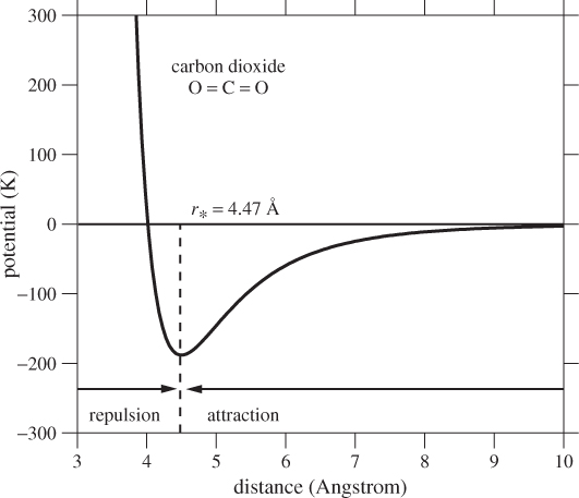
Figure 1-3: Approximate interaction potential between two CO₂ molecules as a function of their separation distance. The potential is given in kelvin; to convert to joule multiply by the Boltzmann constant, k_B = 1.38 × 10⁻²³ J/K. The arrows show the direction of the force on the test molecule in the regions to the left and to the right of r_*.

That is, the magnitude of the force is equal to the slope of the potential with a negative sign that indicates that the force vector points in the direction in which the potential decreases. To visualize the force, we place one molecule at the origin and a test molecule at distance r. The magnitude of the force on the test molecule is equal to the derivative of the potential at that point (the force on the first molecule is equal in magnitude and opposite in direction). If the direction of force is towards the origin, the force is attractive, otherwise it is repulsive. The potential in Figure 1-3 has a minimum at separation distance r_* = 4.47 Å. In the region r > r_* the slope is positive and the force is attractive. The attraction is weaker at longer distances and for r larger than about 9 Å the potential is practically flat and the force is zero. In the region r < r_* the potential is repulsive and its steep slope indicates a very strong force that arises from the repulsive interaction of the electrons surrounding the molecules. Since the molecules cannot be pushed much closer than about r ≈ r_*, we may regard the distance r_* to be the effective diameter of the molecule.¹ Of course, even simple molecules like argon are not solid spheres; therefore, the notion of a molecular diameter should not be taken literally.

1. The closest center-to-center distance we can bring two solid spheres is equal to the sum of their radii. For equal spheres, this distance is equal to their diameter.

The details of the potential vary among different molecules but the general features are always the same: Interaction is strongly repulsive at very short distance, weakly attractive at distance of the order of several Å, and zero at much larger distances. These features help to explain many aspects of the macroscopic behavior of matter.

Temperature and Pressure

In the classical view of molecular phenomena, molecules are small material objects that move according to Newton’s laws of motion, under the action of forces they exert on each other through the potential interaction. Molecules that collide with the container walls are reflected back, and the force of this collision gives rise to pressure. Molecules also collide among themselves,² and during these collisions they exchange kinetic energy. In a thermally equilibrated system, a molecule has different energies at different times, but the distribution of energies is overall stationary and the same for all molecules. Temperature is a parameter that characterizes the distribution of energies inside a system that is in equilibrium with its surroundings. With increasing temperature, the energy content of matter increases. Temperature, therefore, can be treated as a measure of the amount of energy stored inside matter.

2. Molecular collisions do not require solid contact as macroscopic objects do. If two molecules come close enough in distance, the steepness of the potential produces a strong repulsive force that causes their trajectories to deflect.

Phase Transitions

The minimum of the potential represents a stable equilibrium point. At this distance, the force between two molecules is zero and any small deviations to the left or to the right produce a force that points back to the minimum. A pair of molecules trapped at this distance r_* would form a stable pair if it were not for their kinetic energy, which allows them to move and eventually escape from the minimum. The lifetime of a trapped pair depends on temperature. At high temperature, energies are higher, and the probability that a pair will remain trapped is low. At low temperature a pair can survive long enough to trap additional molecules and form a small cluster of closely packed molecules. This cluster is a nucleus of the liquid phase and can grow by further collection to form a macroscopic liquid phase. Thus we have a molecular view of vapor-liquid equilibrium. This picture highlights the fact that to observe a vapor-liquid transition, the molecular potential must exhibit a combination of strong repulsion at short distances with weak attraction at longer distances. Without strong repulsion, nothing would prevent matter from collapsing into a single point; without attraction, nothing would hold a liquid together in the presence of a vapor. We can also surmise that molecules that are characterized by a deeper minimum (stronger attraction) in their potential are easier to condense, whereas a shallower minimum requires lower temperature to produce a liquid. For this reason, water, which associates via hydrogen bonding (attraction) is much easier to condense than say, argon, which is fairly inert and interacts only through weak van der Waals attraction.

Ideal-Gas State

Figure 1-3 shows that at distances larger than about 10 Å the potential of carbon dioxide is fairly flat and the molecular force nearly zero. If carbon dioxide is brought to a state such that the mean distance between molecules is more than 10 Å we expect that molecules would hardly register the presence of each other and would largely move independently of each other, except for brief close encounters. This state can be reproduced experimentally by decreasing pressure (increasing volume) while keeping temperature the same. This is called the ideal-gas state. It is a state—not a gas—and is reached by any gas when pressure is reduced sufficiently. In the ideal-gas state molecules move independently of each other and without the influence of the intermolecular potential. Certain properties in this state become universal for all gases regardless of the chemical identity of their molecules. The most important example is the ideal-gas law, which describes the pressure-volume-temperature relationship of any gas at low pressures.

1.2 Statistical versus Classical Thermodynamics

Historically, a large part of thermodynamics was developed before the emergence of atomic and molecular theories of matter. This part has come to be known as classical thermodynamics and makes no reference to molecular concepts. It is based on two basic principles (“laws”) and produces a rigorous mathematical formalism that provides exact relationships between properties and forms the basis for numerical calculations. It is a credit to the ingenuity of the early developers of thermodynamics that they were capable of developing a correct theory without the benefit of molecular concepts to provide them with physical insight and guidance. The limitation is that classical thermodynamics cannot explain why a property has the value it does, nor can it provide a convincing physical explanation for the various mathematical relationships. This missing part is provided by statistical thermodynamics. The distinction between classical and statistical thermodynamics is partly artificial, partly pedagogical. Artificial, because thermodynamics makes physical sense only when we consider the molecular phenomena that produce the observed behaviors. From a pedagogical perspective, however, a proper statistical treatment requires more time to develop, which leaves less time to devote to important engineering applications. It is beyond the scope of this book to provide a bottom-up development of thermodynamics from the molecular level to the macroscopic. Instead, our goal is to develop the knowledge, skills, and confidence to perform thermodynamic calculations in chemical engineering settings. We will use molecular concepts throughout the book to shed light to new concepts but the overall development will remain under the general umbrella of classical thermodynamics. Those who wish to pursue the connection between the microscopic and the macroscopic in more detail, a subject that fascinated some of the greatest scientific minds, including Einstein, should plan to take an upper-level course in statistical mechanics from a chemical engineering, physics, or chemistry program.

The Laws of Classical Thermodynamics

Thermodynamics is built on a small number of axiomatic statements, propositions that we hold to be true on the basis of our experience with the physical world. Statistical and classical thermodynamics make use of different axiomatic statements; the axioms of statistical thermodynamics have their basis on statistical concepts; those of classical thermodynamics are based on behavior that we observe macroscopically. There are two fundamental principles in classical thermodynamics, commonly known as the first and second law.³ The first law expresses the principle that matter has the ability to store energy within. Within the context of classical thermodynamics, this is an axiomatic statement since its physical explanation is inherently molecular. The second law of thermodynamics expresses the principle that all systems, if left undisturbed, will move towards equilibrium –never away from it. This is taken as an axiomatic principle because we cannot prove it without appealing to other axiomatic statements. Nonetheless, contact with the physical world convinces us that this principle has the force a universal physical law.

3. The term law comes to us from the early days of science, a time during which scientists began to recognize mathematical order behind what had seemed up until then to be a complicated physical world that defies prediction. Many of the early scientific findings were known as “laws,” often associated with the name of the scientist who reported them, for example, Dalton’s law, Ohm’s law, Mendel’s law, etc. This practice is no longer followed. For instance, no one refers to Einstein’s famous result, E = mc², as Einstein’s law.

Other laws of thermodynamics are often mentioned. The “zeroth” law states that, if two systems are in thermal equilibrium with a third system, they are in equilibrium with each other. The third law makes statements about the thermodynamic state at absolute zero temperature. For the purposes of our development, the first and second law are the only two principles needed in order to construct the entire mathematical theory of thermodynamics. Indeed, these are the only two equations that one must memorize in thermodynamics; all else is a matter of definitions and standard mathematical manipulations.

The “How” and the “Why” in Thermodynamics

Engineers must be skilled in the art of how to perform the required calculations, but to build confidence in the use of theoretical tools it is also important to have a sense why our methods work. The “why” in thermodynamics comes from two sources. One is physical: the molecular picture that gives meaning to “invisible” quantities such as heat, temperature, entropy, equilibrium. The other is mathematical and is expressed through exact relationships that connect the various quantities. The typical development of thermodynamics goes like this:

(a) Use physical principles to establish fundamental relationships between key properties. These relationships are obtained by applying the first and second law to the problem at hand.

(b) Use calculus to convert the fundamental relationships from step (a) into useful expressions that can be used to compute the desired quantities.

Physical intuition is needed in order to justify the fundamental relationships in step (a). Once the physical problem is converted into a mathematical one (step [b]), physical intuition is no longer needed and the gear must shift to mastering the “how.” At this point, a good handle of calculus becomes indispensable, in fact, a prerequisite for the successful completion of this material. Especially important is familiarity with functions of multiple variables, partial derivatives and path integrations.

1.3 Definitions

System

The system is the part of the physical world that is the object of a thermodynamic calculation. It may be a fixed amount of material inside a tank, a gas compressor with the associated inlet and outlet streams, or an entire chemical plant. Once the system is defined, anything that lies outside the system boundaries belongs to the surroundings. Together system and surroundings constitute the universe. A system can interact with its surroundings by exchanging mass, heat, and work. It is possible to construct the system in such way that some exchanges are allowed while others are not. If the system can exchange mass with the surroundings it called open, otherwise it is called closed. If it can exchange heat with the surroundings it is called diathermal, otherwise it is called adiabatic. A system that is prevented from exchanging either mass, heat, or work is called isolated. The universe is an isolated system.

A simple system is one that has no internal boundaries and thus allows all of its parts to be in contact with each other with respect to the exchange of mass, work, and heat. An example would be a mole of a substance inside a container. A composite system consists of simple systems separated by boundaries. An example would be a box divided into two parts by a firm wall. The construction of the wall would determine whether the two parts can exchange mass, heat, and work. For example, a permeable wall would allow mass transfer, a diathermal wall would allow heat transfer, and so on.

Equilibrium

It is an empirical observation that a simple system left undisturbed, in isolation of its surroundings, must eventually reach an ultimate state that does not change with time. Suppose we take a rigid, insulated cylinder, fill half of it with liquid nitrogen at atmospheric pressure and the other half with hot, pressurized nitrogen, and place a wall between the two parts to keep them separate. Then, we rupture the wall between the two parts and allow the system to evolve without any disturbance from the outside. For some time the system will undergo changes as the two parts mix. During this time, pressure and temperature will vary, and so will the amounts of liquid and vapor. Ultimately, however, the system will reach a state in which no more changes are observed. This is the equilibrium state.

Equilibrium in a simple system requires the fulfillment of three separate conditions:

1. Mechanical equilibrium: demands uniformity of pressure throughout the system and ensures that there is no net work exchanged due to pressure differences.

2. Thermal equilibrium: demands uniformity of temperature and ensures no net transfer of heat between any two points of the system.

3. Chemical equilibrium: demands uniformity of the chemical potential and ensures that there is no net mass transfer from one phase to another, or net conversion of one chemical species into another by chemical reaction.

The chemical potential will be defined in Chapter 7.

Although equilibrium appears to be a static state of no change, at the molecular level it is a dynamic process. When a liquid is in equilibrium with a vapor, there is continuous transfer of molecules between the two phases. On an instantaneous basis the number of molecules in each phase fluctuates; overall, however, the molecular rates to and from each phase are equal so that, on average, there is no net transfer of mass from one phase to the other.

Constrained Equilibrium

If we place two systems into contact with each other via a wall and isolate them from the rest of their surroundings, the overall system is isolated and composite. At equilibrium, each of the two parts is in mechanical, thermal, and chemical equilibrium at its own pressure and temperature. Whether the two parts establish equilibrium with each other will depend on the nature of the wall that separates them. A diathermal wall allows heat transfer and the equilibration of temperature. A movable wall (for example, a piston) allows the equilibration of pressure. A selectively permeable wall allows the chemical equilibration of the species that are allowed to move between the two parts. If a wall allows certain exchanges but not others, equilibrium is established only with respect to those exchanges that are possible. For example, a fixed conducting wall allows equilibration of temperature but not of pressure. If the wall is fixed, adiabatic, and impermeable, there is no exchange of any kind. In this case, each part establishes its own equilibrium independently of the other.

Extensive and Intensive Properties

In thermodynamics we encounter various properties, for example, density, volume, heat capacity, and others that will be defined later. In general, property is any quantity that can be measured in a system at equilibrium. Certain properties depend on the actual amount of matter (size or extent of the system) that is used in the measurement. For example, the volume occupied by a substance, or the kinetic energy of a moving object, are directly proportional to the mass. Such properties will be called extensive. Extensive properties are additive: if an amount of a substance is divided into two parts, one of volume V₁ and one of volume V₂, the total volume is the sum of the parts, V₁ + V₂. In general, the total value of an extensive property in a system composed of several parts is the sum of its parts. If a property is independent of the size of the system, it will be called intensive. Some examples are pressure, temperature, density. Intensive properties are independent of the amount of matter and are not additive.

As a result of the proportionality that exists between extensive properties and amount of material, the ratio of an extensive property to the amount of material forms an intensive property. If the amount is expressed as mass (in kg or lb), this ratio will be called a specific property; if the amount is expressed in mole, it will be called a molar property. For example, if the volume of 2 kg of water at 25 °C, 1 bar, is measured to be 2002 cm³, the specific volume is

and the molar volume is

In general for any extensive property F we have a corresponding intensive (specific or molar) property:

The relationship between specific and molar property is

where M_m is the molar mass (kg/mol).

State of Pure Component

Experience teaches that if we fix temperature and pressure, all other intensive properties of a pure component (density, heat capacity, dielectric constant, etc.) are fixed. We express this by saying that the state of a pure substance is fully specified by temperature and pressure. For the molar volume V, for example, we write

which reads “V is a function of T and P.” The term state function will be used as a synonym for “thermodynamic property.” If eq. (1.5) is solved for temperature, we obtain an equation of the form

which reads “T is a function of P and V.” It is possible then to define the state using pressure and molar volume as the defining variables, since knowing pressure and volume allows us to calculate temperature. Because all properties are related to pressure and temperature, the state may be defined by any combination of two intensive variables, not necessarily T and P. Temperature and pressure are the preferred choice, as both variables are easy to measure and control in the laboratory and in an industrial setting. Nonetheless, we will occasionally consider different sets of variables, if this proves convenient.

State of Multicomponent Mixture

The state of a multicomponent mixture requires the specification of composition in addition to temperature and pressure. Mixtures will be introduced in Chapter 8. Until then the focus will be on single components.

Process and Path

The thermodynamic plane of pure substance is represented by two axes, T and P. A point on this plane represents a state, its coordinates corresponding to the temperature and pressure of the system. The typical problem in thermodynamics involves a system undergoing a change of state: a fixed amount of material at temperature T_A and pressure P_A is subjected to heating/cooling, compression/expansion, or other treatments to final state (T_C, P_C). A change of state is called a process. On the thermodynamic plane, a process is depicted by a path, namely, a line of successive states that connect the initial and final state (see Figure 1-6). Conversely, any line on this plane represents a process that can be realized experimentally. Two processes that are represented by simple paths on the TP plane are the constant-pressure (or isobaric) process, and the constant-temperature (or isothermal) process. The constant-pressure process is a straight line drawn at constant pressure (path AB in Figure 1-6); the constant-temperature process is drawn at constant temperature (path BC). Any two points on the TP plane can be connected using a sequence of isothermal and isobaric paths.

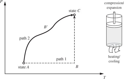
Figure 1-6: Illustration of two different paths (ABC, AB′C) between the same initial (A) and final (C) states. Paths can be visualized as processes (heating/cooling, compression/expansion) that take place inside a cylinder fitted with a piston.

Processes such as the constant-pressure, constant-temperature, and constant-volume process are called elementary. These are represented by simple paths during which one state variable (pressure, temperature, volume) is held constant. They are also simple to conduct experimentally. One way to do this is using a cylinder fitted with a piston. By fitting the piston with enough weights we can exert any pressure on the contents of the cylinder, and by making the piston movable we allow changes of volume due to heating/cooling to take place while keeping the pressure inside the cylinder constant. To conduct an isothermal process we employ the notion of a heat bath, or heat reservoir. Normally, when a hot system is used to supply heat to a colder one, its temperature drops as a result of the transfer of heat. If we imagine the size of the hot system to approach infinity, any finite transfer of heat to (or from) another system represents an infinitesimal change for the large system and does not change its temperature by any appreciable amount. The ambient air is a practical example of a heat bath with respect to small exchanges of heat. A campfire, for example, though locally hot, has negligible effect on the temperature of the air above the campsite. The rising sun, on the other hand, changes the air temperature appreciably. Therefore, the notion of an “infinite” bath must be understood as relative to the amount of heat that is exchanged. A constant-temperature process may be conducted by placing the system into contact with a heat bath. Additionally, the process must be conducted in small steps to allow for continuous thermal equilibration. The constant-volume process requires that the volume occupied by the system remain constant. This can be easily accomplished by confining an amount of substance in a rigid vessel that is completely filled. Finally, the adiabatic process may be conducted by placing thermal insulation around the system to prevent the exchange of heat.

We will employ cylinder-and-piston arrangement primarily as a mental device that allows us to visualize the mathematical abstraction of a path as a physical process that we could conduct in the laboratory.

Quasi-Static Process

At equilibrium, pressure and temperature are uniform throughout the system. This ensures a well-defined state in which, the system is characterized by a single temperature and single pressure, and represented by a single point on the PT plane. If we subject the system to a process, for example, heating by placing it into contact with a hot source, the system will be temporarily moved away from equilibrium and will develop a temperature gradient that induces the necessary transfer of heat. If the process involves compression or expansion, a pressure gradient develops that moves the system and its boundaries in the desired direction. During a process the system is not in equilibrium and the presence of gradients implies that its state cannot be characterized by a single temperature and pressure. This introduces an inconsistency in our depiction of processes as paths on the TP plane, since points on this plane represent equilibrium states of well-defined pressure and temperature. We resolve this difficulty by requiring the process to take place in a special way, such that the displacement of the system from equilibrium is infinitesimally small. A process conducted in such manner is called quasi static. Suppose we want to increase the temperature of the system from T₁ to T₂. Rather than contacting the system with a bath at temperature T₂, we use a bath at temperature T₁ + δT, where δT is a small number, and let the system equilibrate with the bath. This ensures that the temperature of the system is nearly uniform (Fig. 1-7). Once the system is equilibrated to temperature T₁ + δT, we place it into thermal contact with another bath at temperature T₁ + 2δT, and repeat the process until the final desired temperature is reached. Changes in pressure are conducted in the same manner. In general, in a quasi-static process we apply small changes at a time and wait between changes for the system to equilibrate. The name derives from the Latin quasi (“almost”) and implies that the process occurs as if the system remained at a stationary equilibrium state.

Figure 1-7: (a) Typical temperature gradient in heat transfer. (b) Heat transfer under small temperature difference. (c) Quasi-static idealization: temperatures in each system are nearly uniform and almost equal to each other.

Quasi Static is Reversible

A process that is conducted in quasi-static manner is essentially at equilibrium at every step along the way. This implies that the system can retrace its path if all inputs (temperature and pressure differences) reverse sign. For this reason, the quasi-static process is also a reversible process. If a process is conducted under large gradients of pressure and temperature, it is neither quasi static nor reversible. Here is an exaggerated example that demonstrates this fact. If an inflated balloon is punctured with a sharp needle, the air in the balloon will escape and expand to the conditions of the ambient air. This process is not quasi static because expansion occurs under a nonzero pressure difference between the air in the ballon and the air outside. It is not reversible either: we cannot bring the deflated balloon back to the inflated state by reversing the action that led to the expansion, i.e., by “de-puncturing” it. We can certainly restore the initial state by patching the balloon and blowing air into it, but this amounts to performing an entirely different process. The same is true in heat transfer. If two systems exchange heat under a finite (nonzero) temperature difference, as in Figure 1-7(a), reversing ΔT is not sufficient to cause heat to flow in the reverse direction because the temperature gradient inside system 1 continues to transfer heat in the original direction. For a certain period of time the left side of system 1 will continue to receive heat until the gradient adjusts to the new temperature of system 2. Only when a process is conducted reversibly is it possible to recover the initial state by exactly retracing the forward path in the reverse direction. The quasi-static way to expand the gas is to perform the process against an external pressure that resists the expansion and absorbs all of the work done by the expanding gas. To move in the forward direction, the external pressure would have to be slightly lower than that of the gas; to move in the reverse direction, it would have to be slightly higher. In this manner the process, whether expansion or compression, is reversible. The terms quasi static and reversible are equivalent but not synonymous. Quasi static refers to how the process is conducted (under infinitesimal gradients); reversible refers to the characteristic property that such process can retrace its path exactly. The two terms are equivalent in the sense that if we determine that a process is conducted in a quasi-static manner we may conclude that it is reversible, and vice versa. In practice, therefore, the two terms may be used interchangeably.

1.4 Units

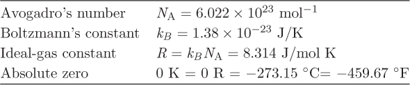
Throughout this book we will use primarily the SI system of units with occasional use of the American Engineering system. The main quantities of interests are pressure, temperature, and energy. These are briefly reviewed below. Various physical constants that are commonly used in thermodynamics are shown in Table 1-1.

Table 1-1: Thermodynamic constants

Pressure

Pressure is the ratio of the force acting normal to a surface, divided by the area of the surface. In thermodynamics, pressure generates the forces that give rise to mechanical work. The SI unit of pressure is the pascal, Pa, and is defined as the pressure generated by 1 N (newton) acting on a 1 m² area:

The last equality in the far right is obtained by writing J = N · m. The pascal is an impractically small unit of pressure because 1 N is a small force and 1 m² is a large area. A commonly used multiple of Pa is the bar:

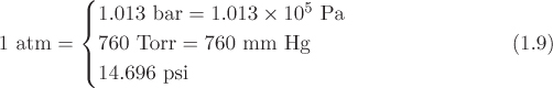
An older unit of pressure, still in use, is the Torr, or mm Hg, representing the hydrostatic pressure exerted by a column of mercury 1 mm high. In the American Engineering system of units, pressure is measured in pounds of force per square inch, or psi. The relationship between the various units can be expressed through their relationship to the standard atmospheric pressure:

Temperature

Temperature is a fundamental property in thermodynamics. It is a measure of the kinetic energy of molecules and gives rise the sensation of “hot” and “cold.” It is measured using a thermometer, a device that obtains temperature indirectly by measuring some property that is a sensitive function of temperature, for example, the volume of mercury inside a capillary (mercury thermometer), the electric current between two different metallic wires (thermocouple), etc. In the SI system, the absolute temperature is a fundamental quantity (dimension) and its unit is the kelvin (K). In the American Engineering system, absolute temperature is measured in rankine (R), whose relationship to the kelvin is,

Temperatures measured in absolute units are always positive. The absolute zero is a special temperature that cannot be reached except in a limiting sense.

In practice, temperature is usually measured in empirical scales that were originally developed before the precise notion of temperature was clear. The two most widely used are the Celsius scale and the Fahrenheit. They are related to each other and to the absolute scales as follows:⁴

4. The notation T/°C reads, “numerical value of temperature expressed in °C.” For example, if T = 25°C, then T/°C is 25.

where the subscript in T indicates the corresponding units. The units of absolute temperature are indicated without the degree (°) symbol, for example, K or R; the units in the Celsius and Fahrenheit scales include the degree (°) symbol, for example, °C, °F. Although temperatures are almost always measured in the empirical scales Celsius or Fahrenheit, it is the absolute temperature that must be used in all thermodynamics equations.

Mole (mol, gmol, lb-mol)

The mole⁵ is a defined unit in the SI system such that 1 mol is an amount of matter that contains exactly N_A molecules, where N_A = 6.022 × 10²³ mol⁻¹ is Avogadro’s number.⁶ The mass of 1 mol is the molar mass and is numerically equal to the molecular weight multiplied by 10⁻³kg. For example, the molar mass of water (molecular weight 18.015) is

5. The symbol of the unit is “mol” but the name of the unit is “mole,” much like the unit of SI temperature is the kelvin but the symbol is K.

6. The units for Avogadro’s number are number of molecules/mol, and since the number of molecules is dimensionless, 1/mol.

The symbol M_m will be used to indicate the molar mass. The number of moles n that correspond to mass m is

The pound-mol (lb-mol) is the analogous unit in the American Engineering system and represents an amount of matter equal to the molecular weight expressed in lbm. The relationship between the mol and lb-mol is

Energy

The SI unit of energy is the joule, defined as the work done by a force 1 N over a distance of 1 m, also equal to the kinetic energy of a mass 1 kg with velocity 1 m/s:

The kJ (1 kJ = 1000 J) is a commonly used multiple.

As a form of energy, heat does not require its own units. Nonetheless, units specific to heat remain in wide use today, even though they are redundant and require additional conversions when the calculation involves both heat and work. These units are the cal (calorie) and the Btu (British thermal unit) and are related to the joule through the following relationships:

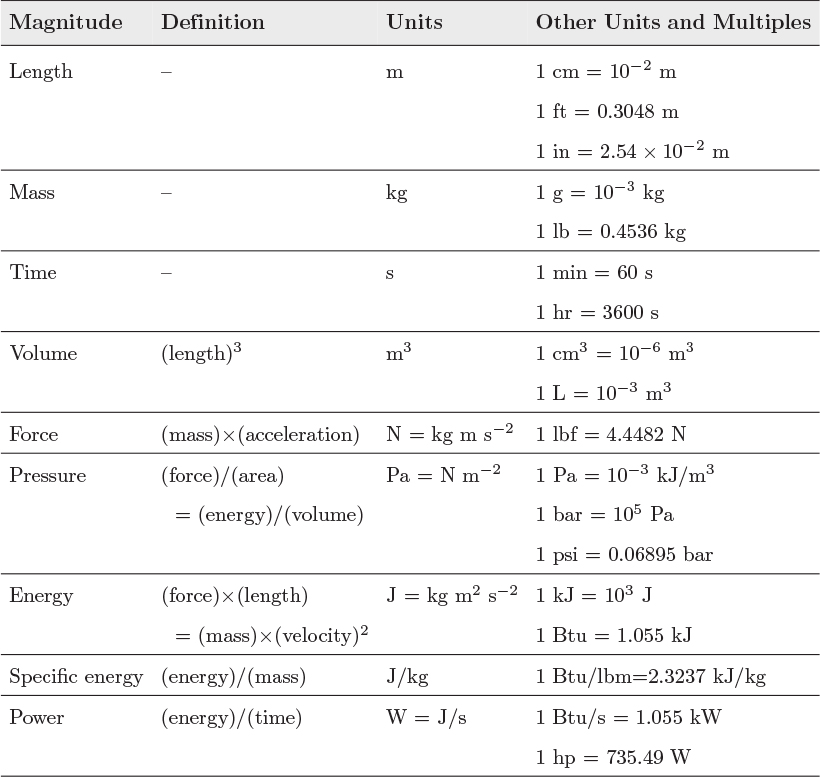
Some unit conversions encountered in thermodynamics are shown in Table 1-2.

Table 1-2: Common units and conversion factors

1.5 Summary

Thermodynamics arises from the physical interaction between molecules. This interaction gives rise to temperature as a state variable, which, along with pressure, fully specifies the thermodynamic state of a pure substance. Given pressure and temperature, all intensive properties of a pure substance are fixed. This means that we can measure them once and tabulate them as a function of pressure and temperature for future use. Such tabulations exist for many substances over a wide range of conditions. Nonetheless, for engineering calculations it is convenient to express properties as mathematical functions of pressure and temperature. This eliminates the need for new experimental measurements—and all the costs associated with raw materials and human resources—each time a property is needed at conditions that are not available from tables. One goal of chemical engineering thermodynamics is to provide rigorous methodologies for developing such equations.

Strictly speaking, thermodynamics applies to systems in equilibrium. When we refer to the pressure and temperature of a system we imply that the system is in equilibrium so that it is characterized by a single (uniform) value of pressure and temperature. Thermodynamics also applies rigorously to quasi-static processes, which allow the system to maintain a state of almost undisturbed equilibrium throughout the entire process.

1.6 Problems

Problem 1.1: The density of liquid ammonia (NH₃) at 0 °F, 31 psi, is 41.3 lb/ft³.

a) Calculate the specific volume in ft³/lb, cm³/g and m³/kg.

b) Calculate the molar volume in ft³/lbmol, cm³/mol and m³/mol.

Problem 1.2: The equation below gives the boiling temperature of isopropanol as a function of pressure:

where T is in kelvin, P is in bar, and the parameters A, B, and C are

A = 4.57795, B = 1221.423, C = −87.474.

Obtain an equation that gives the boiling temperature in °F, as a function of ln P, with P in psi. Hint: The equation is of the form

but the constants A′, B′, and C′ have different values from those given above.

Problem 1.3: a) At 0.01 °C, 611.73 Pa, water coexists in three phases, liquid, solid (ice), and vapor. Calculate the mean thermal velocity () in each of the three phases in m/s, km/hr and miles per hour.

b) Calculate the mean translational kinetic energy contained in 1 kg of ice, 1 kg of liquid water, and 1 kg of water vapor at the triple point.

c) Calculate the mean translational kinetic energy of an oxygen molecule in air at 0.01 °C, 1 bar.

Problem 1.4: The intermolecular potential of methane is given by the following equation:

with a = 2.05482 × 10⁻²¹ J, σ = 3.786 Å, and r is the distance between molecules (in Å).

a) Make a plot of this potential in the range r = 3 Å to 10 Å.

b) Calculate the distance r_* (in Å) where the potential has a minimum.

c) Estimate the density of liquid methane based on this potential.

Find the density of liquid methane in a handbook and compare your answer to the tabulated value.

Problem 1.5: a) Estimate the mean distance between molecules in liquid water. Assume for simplicity that molecules sit on a regular square lattice.

b) Repeat for steam at 1 bar, 200 °C (density 4.6 × 10⁻⁴ g/cm³).

Report the results in Å.

Problem 1.6: In 1656, Otto von Guericke of Magdeburg presented his invention, a vacuum pump, through a demonstration that became a popular sensation. A metal sphere made of two hemispheres (now known as the Magdeburg hemispheres) was evacuated, so that a vacuum would hold the two pieces together. Von Guericke would then have several horses (by one account, 30 of them, in two teams of 15) pulling, unsuccessfully, to separate the hemispheres. The demonstration would end with the opening of a valve that removed the vacuum and allowed the hemispheres to separate. Suppose that the diameter of the sphere is 50 cm and the sphere is completely evacuated. The sphere is hung from the ceiling and you pull the other half with the force of your body weight. Will the hemispheres come apart? Support your answer with calculations.