Chapter 12. Nonideal Solutions
The ideal solution assumes equal strength of self- and cross-interactions between components. When this is not the case, the solution deviates from ideal behavior. Deviations are simple to detect: upon mixing, nonideal solutions exhibit volume changes (expansion or contraction) and exhibit heat effects that can be measured. Such deviations are quantified via the excess properties. An important new property that we encounter in this chapter is the activity coefficient. It is related to the excess Gibbs free energy and is central to the calculation of the phase diagram.
In this chapter you will learn how to:
1. Obtain excess properties (volume, enthalpy, Gibbs free energy) from experimental data.
2. Calculate activity coefficients using an appropriate model.
3. Calculate the phase diagram of nonideal mixtures
12.1 Excess Properties
An excess property is the difference between the property of solution and the same property calculated by the ideal-solution equations:
For the primary properties of interest, volume, enthalpy, and entropy, this definition produces the following results:
Expressions for other properties are obtained similarly. For internal energy we have
Similarly, for the Gibbs free energy the result is
By definition, the excess properties of ideal solution are zero. We may view the excess properties as corrections that must be added to the ideal-solution equations in order to obtain the correct property of solution.
A special case is the limit of pure component, reached when the amount (moles) of component i in the solution is increased indefinitely while keeping all other components constant. In this case, xi → 1 for component i and xj → 0 for all others. According to (12.2)–(12.6), in this limit all excess properties reduce to zero.1 This means that a pure liquid is a special case of ideal solution.2 In a binary solution, a graph of any excess property as a function of x1 meets the zero axis both at x1 = 1 (pure component 1) and at x1 = 0 (pure component 2).
1. The summation ![]() ln xi goes to zero when xi = 1, xj ≠ i = 0.
ln xi goes to zero when xi = 1, xj ≠ i = 0.
2. In a pure liquid the only type of interaction is self-interaction. In this respect, the pure liquid satisfies the ideal-solution condition that all interactions be of equal strength.
Note
Excess Properties as a Mathematical Operator
It is convenient to think of the excess property as a mathematical operator that removes the ideal-solution part from a thermodynamic property. It is a linear operator and can be combined with other operators, such as the partial molar differentiation. Expressions that can be written between regular properties may be written for the excess and for the partial molar excess properties. For example, starting with the fundamental relationship
dG = −SdT + VdP,
which applies to systems of constant composition, we may immediately write the corresponding relationships for the excess and the excess partial molar properties:
In the last equation we have applied both the excess and the partial molar operator. The order in which they are applied does not matter.
Excess Partial Molar Properties
Excess partial molar properties are obtained by applying the partial molar operator on an excess property. Recall that the definition of the partial molar operator is
and involves the differentiation of extensive property Ftot with respect to ni. It is convenient to express partial molar property ![]() as a derivative in terms of xi. In the case of a binary solution, this leads to simple results, as we will see. We begin by obtaining the relationship between derivatives in ni and in xi. Starting with
as a derivative in terms of xi. In the case of a binary solution, this leads to simple results, as we will see. We begin by obtaining the relationship between derivatives in ni and in xi. Starting with
we take the derivative with respect to n1 at constant n2:

We return to the definition of partial molar and expand the right-hand side by applying the chain rule:

Using eq. (12.7) the above results becomes
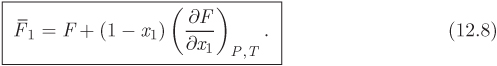
The corresponding expression for the partial molar property of component 2 is obtained by symmetry: exchanging subscripts 1 and 2 we obtain
Using dx2 = −dx1 we obtain ![]() in the equivalent form
in the equivalent form

Here, both partial molar properties are given as derivatives with respect to the mol fraction of component 1. Equations (12.8) and (12.9) apply to any partial molar properties, including excess partial molar. There is a simple graphical interpretation of these equations, as shown in Figure 12-1. In a plot of property F against x1, we draw a tangent line at a mol fraction of interest. The zero intercept of this line is the partial molar property of component 2 and the intercept at x1 is the partial molar of component 1. This is easy to prove if we notice that the tangent line has the equation
where F and ![]() are the values of property F and its derivative at the point of the tangent. At x = 0 it reduces to eq. (12.9), which gives
are the values of property F and its derivative at the point of the tangent. At x = 0 it reduces to eq. (12.9), which gives ![]() ; at x = 1 it reduces to eq. (12.8), which gives
; at x = 1 it reduces to eq. (12.8), which gives ![]() . This graphical construction is useful in determining the partial molar excess properties from experimental data, as demonstrated with the examples below.
. This graphical construction is useful in determining the partial molar excess properties from experimental data, as demonstrated with the examples below.
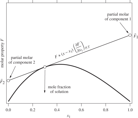
Figure 12-1: Graphical interpretation of partial molar properties in binary mixture.
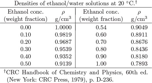
VE = V − xE VE − (1 − xE) VW,
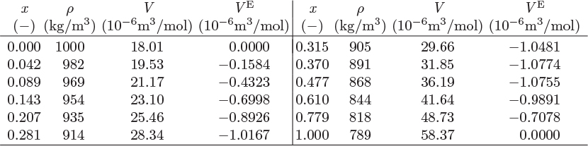
c1 = −6.19944 × 10⁻⁶, c2 = 1.1561 × 10⁻⁵, c3 = −8.6877 × 10⁻⁶, c4 = 3.32617 × 10⁻⁶.
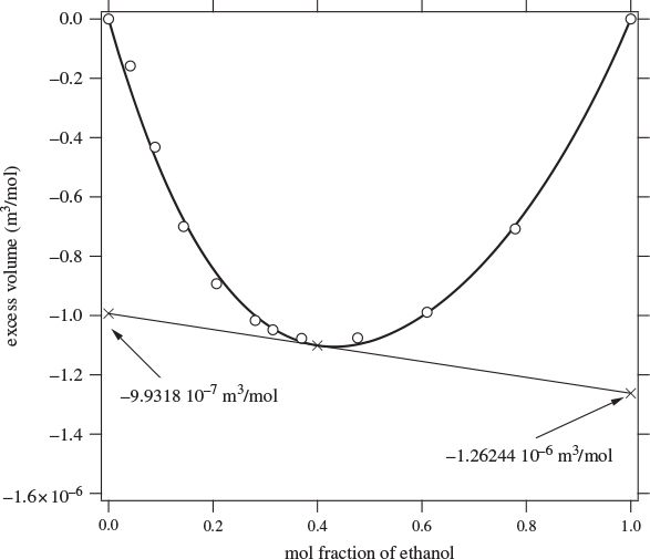
Figure 12-2: Excess volume of ethanol/water solutions at 20 °C (see Example 12.2).

Note
Fitting Excess Properties–Redlich-Kister Expansion
All excess properties of binary solutions must go to zero at x1 = 0 and x1 = 1. One equation that satisfies this condition is
where ci are coefficients, to be obtained by fitting. This polynomial can be written in the more symmetric form as
where ai is a new set of coefficients that are related to the coefficients ci (c0 = a0 − a1 + a2 − ..., c1 = 2a1 − 4a2 + ..., and so on). In the above form, the polynomial is known as the Redlich-Kister expansion and is commonly used to fit experimental data of excess properties, not only volume, but also enthalpy and Gibbs free energy. This is not the only mathematical form used to fit excess properties. Nonpolynomial forms are often necessary with systems that are highly nonideal.
12.2 Heat Effects of Mixing
The mixing of components that form nonideal solution is accompanied by heat effects originating from the fact that the enthalpy of the solution is generally different than the sum of enthalpies of the pure components before mixing. The excess enthalpy of solution is the same as the enthalpy of mixing. It is determined experimentally by calorimetry. If the enthalpy of mixing is positive mixing is endothermic (heat must be added to the solution); if negative mixing is exothermic (heat is rejected by the system to the surroundings). Nonideal systems may exhibit either behavior, or even both behaviors, depending on temperature and composition. Figure 12-3 shows smoothed experimental data for solutions of ethanol in water. This highly nonideal system shifts from exothermic behavior at 323.15 K to endothermic at 373.15 K. The excess enthalpy is a strong function of composition and temperature. It is not possible generally to describe these dependences by a single equation. The typical approach is to fit the experimental data at each temperature to an expression with enough terms to obtain good accuracy. Pressure, on the other hand, has negligible effect.
If the excess enthalpy is known, energy balances can be performed. The starting point for such calculations is eq. (12.3), which for binary solution becomes
H = x1H1 + x2H2 + HE.
The enthalpies of pure liquid components, H1 and H2, are calculated by any of the methods discussed for pure components; the excess enthalpy is calculated either from graphs, such as Figure 12-3, or from equations fitted to experimental data.
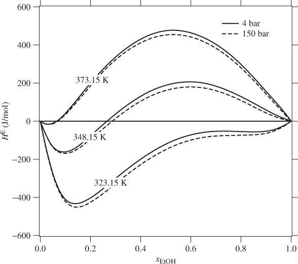
Figure 12-3: Excess enthalpy of ethanol(1)-water(2) solutions (from Ott et al., J. Chem. Thermodynamics, 18[1986], pp. 867–875).
Q = HE = −403 J/mol.
Q = 0 = ΔH,
H(T′) = x1H1(T′) + x2H2(T′) + HE(T′).
CP1 = 123.1 J/mol K, CP2 = 75.2 J/mol K.
HE(323.15 K) = −403 J/mol, HE(348.15 K) = − 76 J/mol,
H = Hid + HE.
Hid = x1H1 + x2H2.
CP = (0.2)(123.1) + (0.8)(75.2) + (13.0) = 97.8 J/mol K.
Enthalpy Charts
Solution enthalpies are typically presented graphically in the form of excess enthalpies plotted as a function of composition and temperature, such as those in Figure 12-3. From such data we can obtain the enthalpy of solution by adding the excess enthalpy to the ideal-solution enthalpy:
H = x1H1 + x2H2 + HE.
This equation may be used to calculate energy balances, as was done in Example 12.3. The same equation may be used to tabulate the enthalpy of the solution as a function of temperature and composition. Combining with an ideal-mixture treatment of the vapor phase, it is possible then to construct the enthalpy chart over the entire phase region of the mixture. One example of such graph is given in Figure 12-4, which shows the enthalpy of hydrazine/water mixtures as a function of composition over a temperature range that includes solid, liquid, and vapor phases. There is a solid phase near the bottom, a liquid region, shown by the gray area in the lower part of the graph, a vapor region, shown by the gray area at the top, and a vapor-liquid coexistence region in between. Isotherms in the vapor-liquid region are straight lines that connect points on the bubble line (upper boundary of the liquid region) to the dew line (lower boundary of the vapor region). The linearity in this region is a direct consequence of the lever rule, according to which, the enthalpy of a two-phase mixture is a linear combination of the molar enthalpies in each phase. In the liquid, isotherms are curved due to nonideal interactions between the components.3
3. If the solution were ideal, isotherms in the liquid would be straight lines.

Figure 12-4: Enthalpy of hydrazine/water mixtures (adapted from Tyner, AIChE J. 1, no. 1 [1955], p. 87).
Enthalpy-composition charts simplify enthalpy calculations considerably. Adiabatic mixing, in particular, can be easily solved graphically in such charts. Suppose that a mass mA of solution A with mass fraction xA of component 1 (this is the component plotted on the horizontal axis of the enthalpy-composition chart) is mixed adiabatically with mass mB of solution B that contains mass fraction xB of component 1. By mass balance, the composition of the resulting mixture (C) is
where w = mA/(mA + mB) is the weight fraction of solution A. The energy balance is
(mA + mB)HC = mAHA + mBHB,
which, solved for HC, gives
Equations (12.11) and (12.12) are parametric equations of a linear relationship between HC and xC.4 If we let w vary (by varying the relative amounts of solutions A and B) and plot HC against xC, we obtain a straight line that passes from points (xA, HA) and (xB, HB) (see Figure 12-5). This leads to a simple graphical procedure for calculating the temperature of the final state:
4. To prove this, eliminate w between eqs. (12.11) and (12.12) to obtain an equation between HC and xC.
1. Define points A and B on the chart, based on the composition and temperature of the initial solutions.
2. Calculate the composition xC of the final solution.
3. The state of the final solution lies on the straight line AB, at the composition xC calculated above.
4. The temperature of the final solution corresponds to the isotherm that passes through point C.
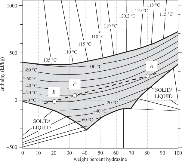
Figure 12-5: Adiabatic mixing of solutions on the enthalpy-composition chart. The initial solutions (A and B) and the solution they produce (C) lie on a straight line. (See Example 12.5.)
This procedure also allows us to determine the phase of the final mixture. If point C lies in the two-phase region, then xC is understood to refer to the overall composition of the mixture. The compositions of the individual phases are obtained from the tie line and once these compositions are known, the amounts of each phase may be calculated using the lever rule. The same procedure works if enthalpy and compositions are given on a molar rather than mass basis.
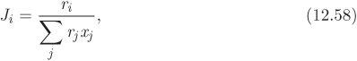
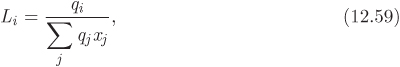
12.3 Activity Coefficient
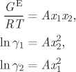
To perform calculations of phase equilibrium we must obtain expressions for the fugacity of component in solution. The key excess property here is the Gibbs free energy of solution. We begin by defining a new dimensionless property, the activity coefficient (γi) of component i in solution:
where ![]() is the excess partial molar Gibbs free energy. Next, we obtain the chemical potential of component in solution. We begin by writing the solution Gibbs free energy in terms of the ideal-solution and the excess free energy,
is the excess partial molar Gibbs free energy. Next, we obtain the chemical potential of component in solution. We begin by writing the solution Gibbs free energy in terms of the ideal-solution and the excess free energy,
G = Gid + GE.
We apply the partial molar operator and notice that on the left-hand side we obtain the chemical potential of component in the solution. The first term on the right-hand side is the chemical potential of the component in ideal solution, and the second term is the excess partial molar Gibbs free energy:
The chemical potential of component in ideal solution is given by eq. (11.9)
where Gi is the molar Gibbs free energy of pure liquid component i, and xi is the mol fraction of component in solution. Combining this result, and making use of the definition of the activity coefficient, the chemical potential of component i in solution takes the form
To calculate the fugacity, we return to eq. (10.18),
which provides the relationship between fugacity and chemical potential. Taking state A to be component i in solution ![]() and B to be component i as the pure liquid
and B to be component i as the pure liquid ![]() , we obtain
, we obtain
or
The usefulness of the activity coefficient should be clear now: it acts as a correction factor in the chemical potential and fugacity and accounts for nonideal interactions between components. Before we study the activity coefficient in more detail, we examine some important limits:
• Ideal Solution. By definition in ideal solution all excess properties are zero. Accordingly, ![]() and the activity coefficient of all components at all compositions are 1. Equations (12.15) and (12.16) then revert to the correct results for ideal solution, eqs. (11.9) and (11.10), respectively.
and the activity coefficient of all components at all compositions are 1. Equations (12.15) and (12.16) then revert to the correct results for ideal solution, eqs. (11.9) and (11.10), respectively.
• Pure Liquid. In the pure liquid all excess properties are zero. It follows that the activity coefficient of a pure liquid is 1. This must also understood to apply in the limiting sense, when the mol fraction of a component is made to approach 1 (by adding large amounts of that component, for example):
• Infinite Dilution. This is the limit approached by the minority species when the mol fraction of the majority species approaches 1. The activity coefficient at this limit is known as the activity coefficient at infinite dilution:
The value of ![]() depends on component i as well as on all other components that are present at this limit.
depends on component i as well as on all other components that are present at this limit.
Activity Coefficient and Excess Gibbs Energy
We return to the definition of the activity coefficient and solve for the excess partial molar Gibbs free energy:
The molar excess Gibbs free energy of solution is obtained by summing up the partial molar contributions of all components:

This equation provides a direct relationship between activity coefficients and excess Gibbs free energy. We return now to eq. (10.5), which we apply to a system of constant composition5
5. Since all ni are constant, we have chosen the total number of moles to be 1. Then the superscript tot can be dropped since we are referring to 1 mol of solution.
Next we apply the partial molar and the excess operator to write
and recognize the right-hand side as the differential of ln γi:

This last result gives the differential of ln γi with respect to temperature and pressure at constant composition and leads to the following identifications,
These partial derivatives quantify the sensitivity of the activity coefficient on temperature and pressure. Since the volume of mixing is generally very small, the effect of pressure on the activity coefficient is small and under typical conditions negligible. Sensitivity on temperature depends on the magnitude of the partial molar enthalpy. For small temperature differences it is common to neglect the effect of temperature and assume the activity coefficient to be constant. This approximation however is inappropriate for systems that are strongly endothermic or exothermic.
Note
Molecular View of Nonideal Effects
In a solution of two components, a molecule is surrounded by a mix of similar and dissimilar molecules and experiences a combination of self- and cross-interactions, as shown schematically in Figure 12-6. The total energy of interaction depends on the average number of neighbors and on how many of them are of the same kind. If self and cross interactions are identical in strength and the two components have similar molecular sizes, we obtain an ideal solution: a molecule is surrounded by the same number of neighbors on average, whether in pure liquid or in solution, and its total interaction with its neighbors does not depend on how many of them are of similar or dissimilar kind. If self and cross interactions are different, the solution environment surrounding a molecule is quite different from the environment in the pure liquid. This causes deviations from ideal-solution behavior. Difference in molecular size is also a source of nonidealities because the arrangement of neighbors around a molecule is affected. In the limit xi → 1, component i approaches ideal-solution behavior because it, interacts almost exclusively with molecules of the same type (component i is the majority component at this limit). In this solution the minority component is found at its infinite dilution limit: a molecule of the minority component is completely surrounded by dissimilar molecules and experience cross interactions only. The activity coefficient of the minority component shows its maximum deviation from 1 at the infinite dilution limit.

Figure 12-6: Molecular view of solution.
Contributions to nonideality that are caused by differences in molecular size are called combinatorial and are related to the arrangement of molecules in space. Contributions that are caused by molecular interactions are called residual. The goal of solution theories is to provide suitable approximations for these two sources of nonideal behavior.
12.4 Activity Coefficient and Phase Equilibrium
To perform VLE calculations, the starting point is the equality of the fugacity of component in the two phases:
For the fugacity of the vapor we use the general expression
where ![]() is the fugacity coefficient of component in the vapor mixture. For the liquid we use eq. (12.16), along with eq. (7.16), which gives the fugacity of the pure liquid:
is the fugacity coefficient of component in the vapor mixture. For the liquid we use eq. (12.16), along with eq. (7.16), which gives the fugacity of the pure liquid:
Combining these results, the vapor-liquid equilibrium condition becomes

This equation is sometimes referred to as the “gamma-phi” method because it uses the fugacity coefficient for the vapor phase and the activity coefficient in the liquid phase. Except for ![]() and γi, all other properties in this equation are those of the pure component. At low pressures we may drop the fugacity coefficients (vapors are assumed to be in the ideal-gas state) and the Poynting correction, which is generally negligible. Under these conditions eq. (12.23) simplifies to
and γi, all other properties in this equation are those of the pure component. At low pressures we may drop the fugacity coefficients (vapors are assumed to be in the ideal-gas state) and the Poynting correction, which is generally negligible. Under these conditions eq. (12.23) simplifies to
Setting γi = 1 (ideal solution) this reverts to Raoult’s law. We may view then the activity coefficient as a correction to Raoult’s law that accounts for deviations from ideal-solution behavior. Equation (12.24) is the basis of VLE calculations, provided that pressure is sufficiently low. It is also used to extract activity coefficients from experimental data, as we will see with examples below.
Positive and Negative Deviations from Raoult’s Law
The activity coefficient appears as a correction factor to Raoult’s law. If γi > 1, the partial pressure of components above the solution are higher than those predicted by Raoult’s law and the solution is said to exhibit positive deviations from ideal-solution behavior. The excess Gibbs free energy is positive in the case (see eq. 12.19). If γi < 1, partial pressures are lower than those predicted by Raoult’s law, the excess Gibbs free energy is negative and the solution is said to exhibit negative deviations. The type of deviation may also be inferred by the general shape of the Pxy graph: under positive deviations, the bubble line lies above the straight line that connects the saturation pressures of the pure components; conversely, under negative deviations the bubble pressure lies below this line. In the special case of ideal solution, the bubble line is a straight line between the saturation pressures. Figure 12-7 shows the Pxy graph, the activity coefficients, and the excess Gibbs free energy for two systems, one that exhibits positive deviations (1,4, dioxane/methanol), and one that exhibits negative deviations (acetone/chloroform). The acetone/chloroform system also exhibits an azeotrope. This is not a necessary feature of systems with negative deviations from ideality.

Figure 12-7: Positive deviations (left) and negative deviations (right) from ideal-solution behavior.
Azeotropes form when deviations from ideality are strong enough, whether these are positive or negative.
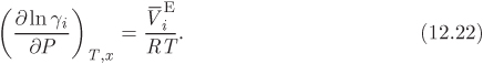
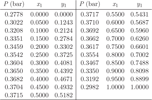
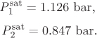
Table 12-1: Pxy data for the system ethanol(1)/acetonitrile(2) at 40 °C (from Sugi H., Katayama T., J. Chem. Eng. Jpn., 11, 167, (1978).)


GE = (8.314 J/mol K)(313.15 K)(0.1524) = 396.78 J/mol.
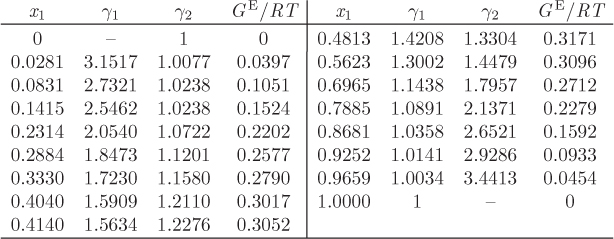
Figure 12-8: Activity coefficients and excess Gibbs energy of ethanol (1)/acetonitrile (2) solutions at 40 °C.
12.5 Data Reduction: Fitting Experimental Activity Coefficients
An equation for the activity coefficient can be obtained by fitting an appropriate equation to the experimental data. Rather than fitting each individual activity coefficient to its own function, the preferred procedure is to fit the excess Gibbs energy as a function x1. The activity coefficients are obtained from this fit by noting from eq. (12.13) that ln γi is in fact a partial molar property; specifically, it is the partial molar property of the ratio GE/RT. As such, ln γi can be obtained from the corresponding molar property of solution by applying eqs. (12.8) and (12.9) with F replaced by GE/RT:

In this approach, a single fitted equation for the excess Gibbs free energy is used to obtain both activity coefficients. This procedure ensures that the fitted activity coefficients are consistent and satisfy the Gibbs-Duhem equation. The challenge is fitting an appropriate mathematical form to the excess Gibbs free energy. From a purely numerical standpoint, the fitted function must be of the form,
which satisfies the condition that the excess Gibbs free energy be zero at x1 = 0 and x1 = 1. The choice of f(x1, x2 = 0 is open. One approach is adopt a Redlich-Kister polynomial,
f(x1, x2) = a0 + a1(x1 − x2) + a2(x1 − x2)2 + ...,
with enough terms to obtain an accurate fit. This approach is satisfactory with some systems but inadequate with others. One of the goals of theory is to provide informed guesses for this unknown function. Based on the assumptions employed, several models have been developed that lead to specific forms for the excess Gibbs energy of solution and the activity coefficients, as discussed in the next section. Before we move to this discussion, we demonstrate the numerical fitting procedure by continuing the example of ethanol/acetonitrile.
a0 = 1.27729, a1 = 0.06540.
γ1 = 2.51046, γ2 = 1.02264.
P = (2.51046)(0.1415)(0.1799 bar) + (1.02264)(1 − 0.1415)(0.2290 bar) = 0.2650 bar.
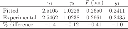
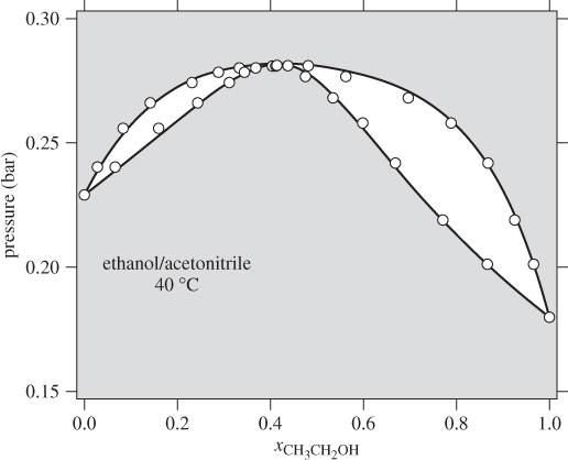
Figure 12-9: Experimental (symbols) and calculated (line) Pxy graph of ethanol/acetonitrile at 40 °C (see Example 12.7).
Note
Data Reduction
The procedure in Examples 12.6 and 12.7 is an example of data reduction: a large set of experimental data (Pxy data) is reduced into an equation for the activity coefficients with two parameters (a0 and a1). The entire Pxy graph may then be reconstructed from these two parameters.
12.6 Models for the Activity Coefficient
Several equations exist for the activity coefficients in nonideal solution. These are based on models for the excess Gibbs free energy of the solution and they are known by the name of the scientists who developed them or by the theory used to model nonideal interactions. The literature on this topic is extensive and remains the subject of research. Here we review some of the most common models that have been used to relate the activity coefficient to composition.
Margules Equation
The Margules equation models the excess Gibbs free energy by a two-parameter Redlich-Kister polynomial. The excess Gibbs energy and the activity coefficients are given by the following equations:
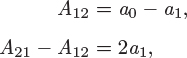
The two constants of the Margules equation bear a simple relationship to the activity coefficients at infinite dilution. Setting x1 = 0 in eq. (12.28) and x2 = 0 in eq. (12.29) we obtain,

You may have noticed that the Margules model is equivalent to the two-parameter Redlich-Kister polynomial used in Example 12.7. This may be confirmed by setting A12 = a0 – a1 and A21 = a0 + a1 to the above equations (see Example 12.8, below). In the form given here, the expressions for the activity coefficients are symmetric in the two components such that each expression is obtained from each other by switching the subscripts 1 and 2.
A simplified form of the Margules equation is obtained if the two parameters are equal. Setting A12 = A21 = A, eqs. (12.27)–(12.29) become
and the activity coefficients at infinite dilution are
From theoretical considerations, this model describes nonideal interactions between molecules of similar molecular size.

A12 = 1.2119, A21 = 1.3427.

Figure 12-10: Linearized form of excess Gibbs free energy in the Margules equation for the system ethanol (1)/acetonitrile (2) at 40 °C (see Example 12.8).
Additional data The saturation pressures are ![]() bar and
bar and ![]() bar.
bar.
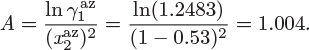
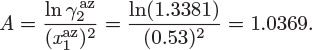
Solution To calculate the value of A in the one-parameter form of the Margules equation we need one experimental value of the activity coefficient. This is obtained from the known azeotropic point. With ![]() we find
we find
van Laar Equation
This model is based on the following equations:

Notice that in this model the excess Gibbs free energy is not a polynomial in the mol fraction. The van Laar equation is a two-parameter model and the constants B12 and B21 are related to the activity coefficients at infinite dilution:
In the special case that B12 = B21, the van Laar model reduces to the same expression as the one-parameter Margules equation (A12 = A21).
Wilson Equation
The Wilson equation is based on local composition theories and accounts for intermolecular interactions between a molecule and its immediate neighbors. The Wilson expression for the excess Gibbs energy and the resulting equations for the activity coefficients are
The two parameters Λ12 and Λ21 are related to molecular properties of the components:
where Vi is the molar volume of the pure component i, and λij is the interaction energy between components i and j (cross interaction if i = j, self-interaction if i ≠ j). In the Wilson model, nonidealities arise from interactions of unequal strength (λii ≠ λij) and from unequal sizes (Vi # Vj). In addition to connecting the excess Gibbs free energy to molecular properties, Wilson’s equation also introduces a temperature dependence of the activity coefficient. The interaction parameters are not known and are usually treated as adjustable parameters, to be obtained by numerical fitting.
Non Random Two Liquid Model (NRTL)
This equation is also based on local composition theories. The expression for the Gibbs free energy is

with
The corresponding activity coefficients are given by
In this equation, gij is the interaction energy (analogous to λij of the Wilson equation). The parameter α arises from the fact that locally the composition of the solution may differ from the bulk concentration giving rise to nonrandom arrangement of molecules. It is usually set to a constant value between 0.2 and 0.3. Treating α as a constant, the NRTL model contains two adjustable parameters, τ12 and τ21 (notice that the individual values of the gij are not needed for the calculation).
Flory-Huggins Model
Polymer-solvent systems differ from usual solutions in that one component (polymer) is much larger than the other (solvent). This leaves less space for the solvent, limits the ways that a chain can stretch in solution and creates a situation where segments of a long polymer chain may be interacting with other segments of the same chain. The Flory-Huggins model accounts for these effects.6 The excess Gibbs energy is given by the expression
6. Paul J. Flory received the 1974 Nobel Prize in Chemistry in recognition of his contributions to polymer science.

Here, 1 refers to the solvent and 2 to the polymer; Φi is the volume fraction of component i, and is defined as
Vi is the molar volume of component i, r is the ratio of the molecular volumes,
and χ is a measure of the interaction energy between polymer and solvent. The corresponding activity coefficients are
The first term in parenthesis on the right-hand side of eq. (12.43) reflects entropic effects that arise from the number of possible ways that macromolecules and solvent can be arranged in space; this term is also known as the combinatorial contribution. The second term on the right-hand side is the enthalpic contribution and arises from differences between polymer-polymer and polymer-solvent interactions; this term is also referred to as the residual contribution (not to be confused with the residual properties introduced earlier, which measure deviations from the ideal-gas state). Even if this term is zero (i.e., χ = 0), the solution is nonideal due to the size difference between polymer and solvent.
UNIQUAC
The name of this model is an acronym of universal quasichemical, the name of the theory used to drive it. Like the Flory-Huggins model, UNIQUAC separates nonideal contributions to the excess Gibbs free energy into a combinatorial and a residual term:
The combinatorial term accounts for differences in size and shape of the molecules and depends entirely on properties of the pure components. The residual term accounts for binary interactions and contains parameters characteristic for a pair of components. For binary solution these are given by the expressions
The activity coefficients are also expressed as a sum of residual and combinatorial contributions,
These terms are given by the following expressions:
with
The corresponding expressions for γ2 are obtained by interchanging the subscripts 1 and 2. The method requires the following parameters: ri, which is a measure of the molecular size of component i, and qi, which represents the surface area of the component, and two binary parameters aij which represent interactions. The parameters ri and qi characterize the pure components and can be calculated from tabulated values. The binary interaction parameters aij represent the difference between the cross-interaction energy, uij and the self-interaction, ujj:
aij = uij − ujj,
(notice that aij ≠ aji). The two aij constants are treated as adjustable parameters and are obtained by fitting eq. (12.46) to experimental data. Assuming aij to be independent of temperature, a single set of these parameters may be used to calculate activity coefficients at other temperatures. UNIQUAC works well with a large variety of nonelectrolyte solutions, including polar components such as water, as well as nonpolar molecules such as hydrocarbons.
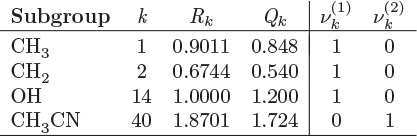
Group Contribution Method for ri, qi
The parameters ri and qi are obtained by the group contribution method, a general approach for the estimation of pure component properties that is based on the premise that a given molecular group makes the same contribution to a property regardless of the molecule to which it is attached. For example, the molecular group CH3 is assumed to make the same contribution to a property (enthalpy, entropy, surface area, etc.) whether it is part of ethane, toluene, or any other molecule. Since there are far fewer molecular groups than there are molecules, the required tabulations are significantly reduced. A number of molecular units, or subgroups, have been identified and their r and q values have been tabulated (see Table D-1 in the appendix). In the nomenclature of UNIFAC, a structural unit is a “subgroup.” Subgroups are grouped together in “main groups.” For instance, CH3, CH2, CH, and C are all subgroups of the main group “CH2.” Each subgroup has been assigned an index value, k, that is unique for that subgroup. For example, k = 9 identifies the subgroup C=C (carbon double bond). To obtain r and q of a molecule, the molecule is broken down in its constituent subgroups and the r and q values are computed as follows:
where ![]() is the number of subgroups of type k that are present in component i, and Qk, Rk, are the corresponding values of the subgroup and are obtained from Table D-1 (in the appendix). Calculations based on the UNIQUAC equation are more involved compared to other methods but the method is appealing because it works well with many nonideal systems. The calculation of the activity coefficients and of the Pxy graph are demonstrated in the example below.
is the number of subgroups of type k that are present in component i, and Qk, Rk, are the corresponding values of the subgroup and are obtained from Table D-1 (in the appendix). Calculations based on the UNIQUAC equation are more involved compared to other methods but the method is appealing because it works well with many nonideal systems. The calculation of the activity coefficients and of the Pxy graph are demonstrated in the example below.
a12 = 294.5 K, a21 = − 41.3 K.
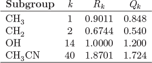
r1 = (1)(0.9011) + (1)(0.6744) + (1)(1.000) = 2.5755,
q1 = (1)(0.848) + (1)(0.540) + (1)(1.200) = 2.588,
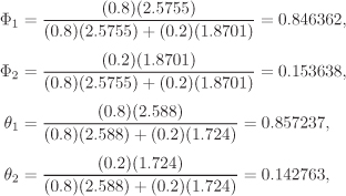
τ12 = exp(− 294.5/318.15) = 0.390454,
12 = exp(− (− 41.3)/318.15) = 1.14098.

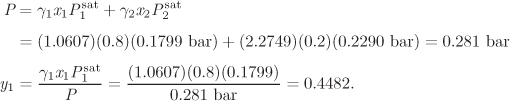
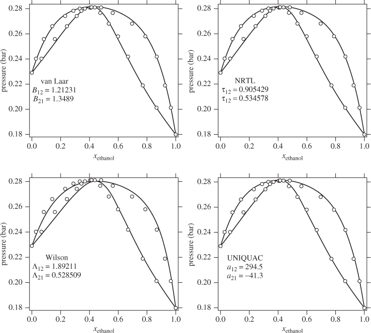
Figure 12-11: Calculated Pxy graphs for the system ethanol/acetonitrile at 40 °C using various activity coefficient models. The parameters have been fitted to the experimental points for the excess Gibbs free energy of solution.
UNIFAC
This method deserves special mention because, unlike all of the previous methods, it allows the prediction of activity coefficients based entirely on tabulated parameters i.e., no fitting of parameters is necessary. It builds on UNIQUAC and is based on the premise that a solution may be regarded as a mixture of structural units rather than of chemical species. For example, a mixture of n-pentane and n-heptane is considered as a mixture of CH2 and CH3 subgroups and so is a mixture of cyclohexane and ethane. In this approach, interaction parameters are determined between a finite number of subgroups and are tabulated. It is then possible to calculate activity coefficients for any solution, binary or multicomponent, from a relatively small number of tabulated values. This is the main advantage of the method. Its applicability is limited to components that are liquid at 25 °C. Parameters for the UNIFAC equation have been determined by fitting a large body of experimental values so as to obtain good agreement for as many experimental systems as possible. As a result, some systems are predicted better than others. At the moment, however, this is the method most extensively used that is capable of predicting the activity coefficient.
UNIFAC (Universal Functional Activity Coefficient) applies the UNIQUAC equation to a solution of subgroups to calculate the combinatorial and the residual contributions. In UNIFAC, these represent interactions among the subgroups rather than among the molecules themselves. The method requires a set of size and surface area constants Rk and Qk for each subgroup k and a set of interaction parameters amk for each pair of subgroups. The size and surface-area tables are the same as those used by UNIQUAC.7 Table D-1 in the appendix shows these values for 44 standard subgroups. Interactions are tabulated by groups, rather than subgroups (i.e., all subgroups within a main group have the same interaction energy). As in UNIQUAC, the interaction parameter amn is not equal to anm.
7. In UNIQUAC, these tables are used to calculate the size and area parameters of the components that form the solution; in UNIFAC, these values are used directly in the calculation of the activity coefficients.
To perform a UNIFAC calculation we must first determine ![]() , the number of functional subgroups of type k that appear in the chemical formula of species i. Also needed are the mole fractions in the solution and temperature. The activity coefficient in UNIFAC is calculated by adding the contributions of the combinatorial term, (γC), and the residual term, (γR):
, the number of functional subgroups of type k that appear in the chemical formula of species i. Also needed are the mole fractions in the solution and temperature. The activity coefficient in UNIFAC is calculated by adding the contributions of the combinatorial term, (γC), and the residual term, (γR):
These terms are calculated by the following set of equations:

The various terms are explained below:
The above equations may be used with any number of components.8 The procedure is tedious for hand calculations but easily automated for computer calculations. Tables listing several subgroups and the corresponding Rk and Qk values are given in Table D-1 in the appendix. The table should be consulted before preparing the input for the UNIFAC calculation since some molecules (e.g., water, methanol, acetonitrile) constitute a single subgroup by themselves. The calculation is illustrated in the example below.
8. The extension of UNIFAC to multicomponent solutions is based on the assumption that interaction between multiple components may be obtained from pair interactions between all possible pairs. This means that no additional tabulations are needed for the calculation of multicomponent solutions.
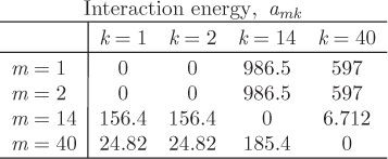
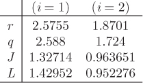
The τmk parameters are calculated as exp(−amk/T):

All other parameters are summarized below:
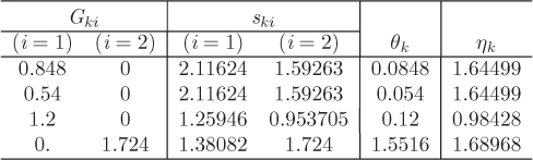
The combinatorial contributions are
and the residual contributions are
γ1 = 2.01244,
γ2 = 1.00918.
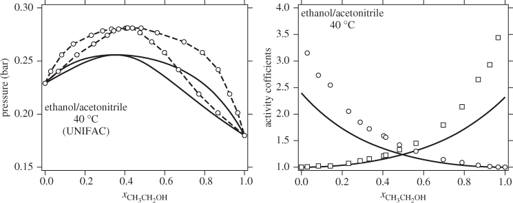
Figure 12-12: Pxy graph and activity coefficients for the system ethanol/acetonitrile at 40 °C calculated from UNIFAC.
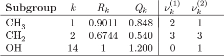
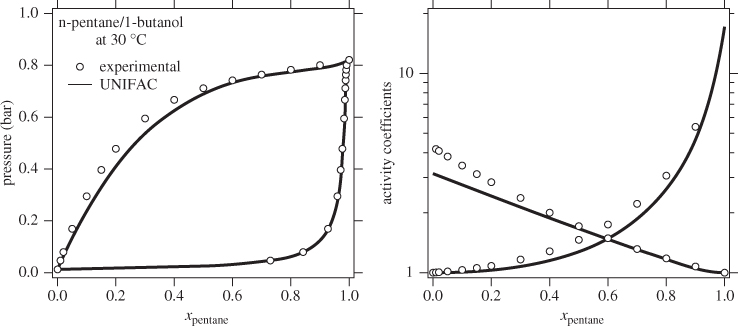
Figure 12-13: Pxy graph and activity coefficients for the system pentane/1-butanol at 30 °C calculated from UNIFAC (data from Ronc and Ratcliff, Can. J. Chem. Eng. 54, no. 326 [1976]).
12.7 Summary
Activity coefficients offer an alternative to equations of state for the calculation of solution properties and vapor-liquid equilibrium. The activity coefficient is closely related to the excess Gibbs free energy, and quantifies deviations from ideal-solution behavior. There is a certain similarity to the fugacity coefficient, which, as we recall, is based on the residual Gibbs free energy and quantifies deviations from the ideal-gas state. The similarity is not coincidental. In both cases we are applying the same basic methodology:9 we adopt an idealized state as our reference state (ideal-gas state, ideal solution) and use appropriate corrections (residual properties, excess properties) to quantify systems that deviated from this idealization. This relationship is depicted schematically in Figure 12-14 and highlights the similarities and differences between calculations based on equations of state and those based on activity coefficients.10 Starting with the ideal-gas state as a reference, deviations are measured via residual properties (partial molar residual, if the target state is the component in solution). These residuals require an equation of state for their calculation. If the reference state is the pure liquid, then deviations are quantified by the excess property (partial molar excess, if the target state is the component in solution). We can now see why the approach based on activity coefficients is so successful: It starts from a reference state that is much closer to the target state. This makes the necessary corrections smaller in magnitude and easier to model. The downside is that these corrections cannot be calculated via purely predictive equations but require input from experiments.
9. The Gibbs free energy is the work that must be done to transfer a molecule from one state to another at constant temperature and pressure. For example, ![]() is the work required to transfer a molecule from an isolated environment of no neighbors (ideal-gas state) into a solution with other molecules.
is the work required to transfer a molecule from an isolated environment of no neighbors (ideal-gas state) into a solution with other molecules.
10. The arrows in Figure 12-14 are drawn qualitatively. In reality, the magnitude of the various Gibbs free energies is in most cases negative.
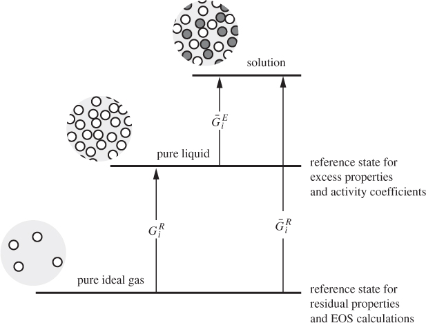
Figure 12-14: Qualitative representation of VLE approach based on equations of state (using residual properties) and approach based on activity coefficients (using excess properties).
The activity coefficient is a correction factor in Raoult’s law that accounts for deviations from ideal-solution behavior. If the activity coefficient is known, VLE calculations can be performed and the phase diagram of the system can be constructed. The activity coefficient depends on temperature, pressure and composition but the most critical variable is composition. The main challenge is how to obtain the activity coefficient for a given system, if experimental data at the desired conditions are not available. Models such as the Margules, van Laar, and the like, provide a correlation between activity coefficients and composition via an equation with a small number of adjustable parameters. These parameters are fitted using experimental data and the agreement between the resulting correlation and the original data is generally very good. UNIFAC contains no adjustable parameters but uses values that have been obtained by regressing a large number of experimental data for several different mixtures. As a result, the accuracy of its predictions varies from system to system. For example, the system n-pentane/1-butanol is predicted fairly accurately, even though it is quite strongly no-ideal (notice the magnitude of the activity coefficients at infinite dilution). By contrast, the system ethanol/acetonitrile is predicted less accurately. The predictive advantage of UNIFAC comes at the expense of accuracy, which is not guaranteed. In the literature we find recommendations that provide decision trees for selecting the appropriate model based on the chemical character of the components. Unfortunately, there is no foolproof method by which to determine which model is best for a given system. The best approach is try various models and validate them against available data before a final choice is made.
12.8 Problems
Problem 12.1: A binary solution is described by the one-parameter equation
where A is constant. At 50 °C and x1 = 0.30 the partial pressures of the two components in the vapor are P1 = 105.3 mm Hg, P2 = 288 mm Hg respectively. The saturation pressure of pure components at 50 °C: P1 = 228 mm Hg, P2 = 380 mm Hg. Calculate the Pxy graph of this system at 50 °C.
Problem 12.2: The table below gives the enthalpy of benzene(1)-heptane(2) solutions at 20 °C 1 bar as a function of the mol fraction of benzene.
a) Calculate and plot the excess enthalpy at 20 °C, 1 bar.
b) Calculate the partial molar excess enthalpy at x1 = 0.2, 20 °C, 1 bar.
c) Calculate the heat that is released or absorbed when 10 mol of benzene is mixed with 40 mol of heptane isothermally at 20 °C, 1 bar.
d) Calculate the temperature change when 10 mol of benzene is mixed with 40 mol of heptane adiabatically, 1 bar, if the initial temperature of the pure components is 20 °C. The heat capacity of the pure liquids are CP1 = 134 J/mol K, CP2 = 222 J/mol K.

Problem 12.3: The table below gives the excess enthalpy for the system acetone(1)-water(2) at 25 °C, 1 bar.
a) Calculate the partial molar enthalpy of each component at x1 = 0.5, 25 °C, 1 bar. The reference state for each component is the pure liquid at 25 °C, 1 bar.
b) Repeat the previous part with the reference state for water changed to the pure liquid at 2 bar,
c) A solution that contains 50% by mole acetone is mixed with equal moles of a solution that contains 80% by mole acetone. The mixing takes place in a heat bath at 25 °C. Determine whether any amount of heat is exchanged between the system and the surroundings. If so, calculate that heat and report whether the mixing is endo- or exothermic.

Problem 12.4: a) Based on Figure 12-5, is the mixing of hydrazine and water an endothermic or exothermic process?
b) Calculate the excess enthalpy for a solution that contains 60% by mol hydrazine at 20 °C.
Problem 12.5: Determine the phase of a mixture of hydrazine and water at 1 bar, 110 °C if the overall mol fraction of hydrazine is 20%. If the state is a mixture of vapor and liquid, report the amounts and compositions in each phase.
(Use Figure 12-5 to answer these questions.)
Problem 12.6: Pure hydrazine is mixed with pure water to form a solution that contains 40% hydrazine (by mol). Both components are initially at 20 °C.
a) Determine the temperature of the final solution if mixing is adiabatic.
b) Determine the amount of heat exchanged with the surroundings if mixing is isothermal.
(Use Figure 12-5 to answer these questions.)
Problem 12.7: The activity coefficients of the system benzene(1)/acetonitrile(2) are given by
At 45 °C, A = 1.
a) Obtain the activity coefficients of the two components at infinite dilution.
b) Does this system form an azeotrope at 45 °C? If so, report the pressure and the azeotropic composition.
c) Calculate the bubble and dew pressure of a system containing 30% benzene by mole at 45 °C.
Additional data. The saturation pressures of components 1 and 2 at 45 °C are 223.7 and 208.4 Torr, respectively.
Problem 12.8: The data in the table below are for the system benzene (1)-diethylamine at 55 °C (Letcher, T. M. and Bayles, J.W., J. Chem. Eng. Data, 16, 266 (1971)):

a) Fit the excess Gibbs energy to a polynomial expression of the form
and obtain the values of a0, a1 and a2.
b) Express the activity coefficients in terms of the above parameters.
c) Make a graph of the Pxy graph calculated from the fitted activity coefficients and compare with the experimental data.
d) Instead of this three parameter fit it has been suggested to use the Margules equation. What is your recommendation?
Problem 12.9: Use the data below for the system benzene(1)/acetonitrile(2) at 45 °C to answer the following questions:
a) What is the saturation pressure of the pure components at 45 °C?
b) What is the phase of the pure components at 45 °C and 34 kPa?
c) Calculate the fugacity of the pure components at the conditions of part (b).
d) Two moles of benzene are mixed with 3 moles of acetonitrile under constant temperature and pressure at 45 °C and 33 kPa. What is the phase of the mixture (vapor, liquid, or mixed)?
e) What is bubble pressure of the mixture at 45 °C?
f) Mark on the graph the points before and after mixing.
g) Calculate the fugacity of the two components at the composition of the azeotrope.
h) Using data from the graph, estimate the activity coefficient of benzene at infinite dilution.
Problem 12.10: The activity coefficients for the system carbon methyl acetate (1)/methanol (2) at 60 °C can be described by the equation
The saturation pressures of the pure components at 60 °C are:
It is also known that at 60 °C the two liquids are fully miscible and that ![]() .
.
a) Does this system exhibit positive or negative deviations from ideality? How can you tell?
b) Calculate the bubble pressure and the composition of the vapor at 60 °C of a solution that contains 63.4% methyl acetate.
c) Calculate the Pxy graph of this system at 60 °C.
Problem 12.11: The laboratory division of your company has sent you the following data for the system n-pentane (1)/propionaldehyde (2) at 35 °C: The activity coefficients of the two components at infinite dilution are 4.0 and the saturation pressures of the pure components are 0.7 and 1 bar, respectively.
a) Does this system exhibit positive, negative, or no deviations from ideal-solution behavior?
b) Assuming the validity of the Margules equation, determine the constants A12 and A21.
c) You suspect that this system forms an azeotrope. What is the composition of the two phases and the pressure at the azeotrope?
d) Draw a qualitative Pxy graph at 35 °C. On the graph show all the information that you have for this system.
e) Your are designing a single flash separation process for a stream that contains 80% n-pentane (the rest is propionaldehyde). The mixture is to be flashed at 35 °C and you must determine the pressure so that the purity of n-pentane is 95%. What is this pressure?
Problem 12.12: At 50 °C the system acetone(1) and chloroform(2) forms an azeotrope with composition x1 = 0.416. The activity coefficients are given by the equation
where A is constant.
a) What is the pressure at the azeotropic composition at 50 °C?
b) One mole of acetone is mixed with one mole of chloroform at 50 °C, 0.5 bar.
What is the phase of the pure components before mixing? What is the phase of the system after mixing?
Additional information: The saturation pressures of the pure components at 50 °C are Pacetone = 0.81 bar, Pchloroform = 0.41 bar.
Problem 12.13: a) Use the data for the system ethyl-methyl ketone(1)-toluene(2) given below (T = 50 °C) to obtain the parameters of the van Laar equation.
b) Reconstruct the Pxy using the van Laar equation and compare with the data.
Problem 12.14: The following data are for the system water(1)/diethylamine(2).
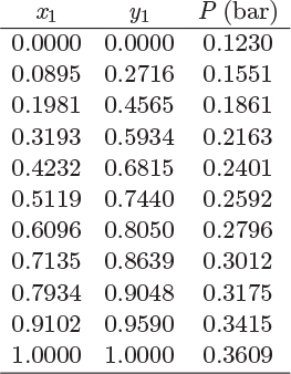
a) Do the components form an ideal solution?
b) Calculate the fugacity and fugacity coefficient of water in a solution that contains 20% water by mole, at the bubble point at 311.5 K.
Problem 12.15: A stream (1) that carries a mixture of heptane (60% by mol) and benzene (40%) is compressed to unspecified pressure (stream 2) in a compressor whose efficiency is 80%. Stream 2 is cooled to 152 °C and the resulting vapor-liquid mixture (stream 3) is separated in a vapor-liquid separator. One of the two streams that exit the separator contains 65% heptane. The activity coefficients for this system are given by the Margules equation with A12 = 3, A21 = 1, where the subscripts 1 and 2, refer to heptane and benzene, respectively. The saturation pressures of heptane and benzene at 152 °C are ![]() , and
, and ![]() , respectively; the ideal heat capacities are CP1 = 208 J/mol K and CP2 = 130 J/mol K. The gas phase may be assumed ideal.
, respectively; the ideal heat capacities are CP1 = 208 J/mol K and CP2 = 130 J/mol K. The gas phase may be assumed ideal.
a) Determine the pressure in all streams.
b) Calculate the molar rates and composition (mol fraction of heptane) in all streams.
c) Calculate the work in the compressor and the temperature of stream 2.
d) Calculate the heat load in the heat exchanger.
e) Calculate the entropy generation for the entire process.
Problem 12.16: The data below are for a vapor/liquid system of two unnamed components:
a) Calculate the activity coefficients of the two components and plot them against x1. Your graph should be done on the computer and it should be properly annotated.
b) Does this system exhibit positive or negative deviations from ideality?
c) Determine whether the system is best described by the Margules or the van Laar equation and determine the parameters of the corresponding equation.
Problem 12.17: The system water (1)/phenol (2) is described by the van Laar equation with B12 = 0.83, B21 = 3.22.
a) Construct the Pxy graph of this system at 100 °C.
b) If a solution that contains 65% (mol) water is flashed to 0.5 bar, 100 °C, what is the composition and relative amounts of the phases that are formed? The saturation pressure of phenol at 100 °C is 0.055 bar.
Problem 12.18: Assuming that the system ethyl methyl ketone (1)/ toluene (2) at 50 °C is described by the Margules equation with A12 = 0.3681, A21 = 0.2046, do the following:
a) Calculate the bubble pressure at 50 °C of a mixture with z1 = 0.3.
b) Calculate the dew pressure at 50 °C of a mixture with z1 = 0.3.
c) A mixture with z1 = 0.3 is flashed to 50 °C at pressure such that a stream is received that contains 88% toluene by mol. Determine the pressure and the percent recovery of toluene in the toluene-rich stream.
Additional information: ![]() ,
, ![]() .
.
Problem 12.19: The following information is available for the system tetrachloro-methane (1) acetic acid (2) at 25 °C:
a) Assuming that the activity coefficients are given by the equations below,
obtain the constants A and B.
b) What is the phase of a system that contains 30% tetrachloromethane, at P = 0.7 bar, T = 25 °C?
c) Calculate the fugacity of tetrachloromethane at the conditions of part (b).
d) Calculate the fugacity coefficient of tetrachloromethane at the conditions of part (a).
e) A mixture of the two components is flashed to conditions that produce a vapor-liquid mixture. The mol fraction of tetrachloromethane in the liquid is x1 = 0.6 and the temperature of the two-phase system is 25 °C. What is the pressure?
f) Calculate the composition of the vapor in the previous part.
g) Calculate the vapor and liquid fractions formed in part (e) if the mol fraction of tetrachloromethane in the initial mixture (before flashing) is 80%.
Problem 12.20: At 70 °C, 1 bar, the system acrylonitrile(1)/water(2) forms two phases with composition, x1A = 0.968, x1W = 0.073, where the subscripts A and W refer to the acrylonitrile-rich and water-rich phases, respectively. Assuming that the Margules equation is appropriate for this system:
a) Calculate the activity coefficients of the two components at the given conditions.
b) Calculate the bubble pressure of the two-phase system at 70 °C and the composition of the vapor.
c) Calculate the Pxy phase diagram at 70 °C.
Additional information: The saturation pressures of the pure components at 70 °C are
Problem 12.21: a) Use the SRK equation to calculate the activity coefficient of oxygen in air (gas) at the dew pressure of air at 120 K.
b) Use the SRK equation to calculate the activity coefficient of oxygen in liquid air at the bubble pressure of air at 120 K.
Assume that air is a mixture of oxygen (21%) and nitrogen (79%) and that k12 = 0.
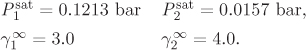
Problem 12.22: The table below shows the results from a VLE calculation for the system normal heptane (1)/normal decane (2) but because someone spilled coffee, some entries are missing.
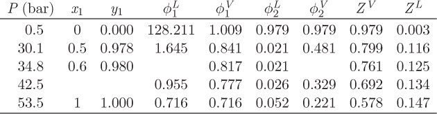
a) Calculate the activity coefficient of n-decane at P = 17.22 bar, T = 570 K, xdecane = 0.7.
b) Is Raoult’s law valid for this system at 570 K? (Answers without justification will not count.)
c) Fill out the missing information in the table. You may not fill out the table by interpolation!
d) Draw a qualitative Pxy graph for this system at 570 K.
e) State and justify your assumptions.
Problem 12.23: The partial molar enthalpies of species 1 and 2 in a binary mixture at 25 °C are given by
where the enthalpy is in kJ/mol of mixture.
a) Calculate the molar enthalpies of the pure components.
b) Calculate the partial molar enthalpies of the two components at infinite dilution.
c) Determine the excess partial molar enthalpies of the two components as functions of the composition and calculate their values at infinite dilution.
d) Calculate the molar enthalpy of an equimolar solution.
e) Calculate the enthalpy change when the two components are mixed at constant temperature and pressure to produce an equimolar solution.
f) Is this an endothermic or exothermic system?
Problem 12.24: Use the UNIFAC equation to estimate the enthalpy of mixing of a solution that contains 37% (mol) acetic acid in water at 20 °C, 1 bar.
Problem 12.25: The infinite dilution activity coefficients of the system water/acetic acid at 100 °C are
a) Obtain the parameters of the Margules equation for this system.
b) Calculate the bubble pressure at 100 °C of a solution with xw = 0.63.
c) Calculate the dew pressure at 100 °C of a solution with xw = 0.63.
Additional data: The Antoine parameters for the two components are:
to be used with
with T in K and Psat in Torr.
Problem 12.26: a) You just finished an SRK calculation for the system carbon dioxide (1) / normal pentane (2) at 290 K when a virus wiped out your hard disk. Fortunately you had printed a copy (see table below), but in your panic to save it, you spilled coffee and can’t make some of the numbers. Fill in the missing entries.
b) How big of a container (cm3) is needed to store 1000 moles of a solution that contains 50% by mole carbon dioxide at 290 K, 30.1 bar?
c) What is the fugacity of carbon dioxide in solution with n-pentane, at x1 = 0.5, T = 290 K, P = 30.1 bar?
d) Calculate the Poynting factor of carbon dioxide in solution with n-pentane, at x1 = 0.5, T = 290 K, P = 30.1 bar.
e) Calculate the activity coefficient of carbon dioxide in the liquid at 50% mole fraction.
f) Does this system obey Raoult’s law at 290 K?
Problem 12.27: Use the UNIFAC equation to do the following calculations for the system methanol(1)-acetic acid(2):
a) Calculate the Pxy graph for this system at 80 °C.
b) Do you expect the volume of the system to expand or to contract upon mixing the pure components?
c) Calculate the fugacity of methanol in mixture with acetic acid at xMeOH = 0.8, 80 °C, 0.4 bar.
d) Repeat the previous calculation at the bubble pressure of the solution instead of 0.4 bar.
e) Calculate the chemical potential of methanol in mixture with acetic acid at xMeOH = 0.8, 80 °C, 0.4 bar. The reference state is the pure liquid at 80 °C, 0.4 bar. How is your answer affected by the fact that methanol is in the vapor phase at 80 °C, 0.4 bar?
f) Repeat the previous part if the reference state is the pure liquid at saturation at 80 °C.
Additional data: The saturation pressures of methanol and acetic acid at 80 °C are 1.81 and 0.2763 bar, respectively.
Problem 12.28: Use the UNIFAC method to calculate the following phase diagrams for the system water(1)-ethanol(2):
a) Pxy graph at 100 °C.
b) Txy graph at 1 bar.
Problem 12.29: Use the UNIFAC equation to calculate the Pxy graph for the system water/acetic acid at 100 °C. The saturation pressure of acetic acid at 100 °C is 0.57 bar.