
Chapter 2. The Energy Balance
When you can measure what you are speaking about, and express it in numbers, you know something about it. When you cannot measure it, your knowledge is meager and unsatisfactory.
Lord Kelvin
The energy balance is based on the postulate of conservation of energy in the universe. This postulate is known as the first law of thermodynamics. It is a “law” in the same sense as Newton’s laws. It is not refuted by experimental observations within a broadly defined range of conditions, but there is no mathematical proof of its validity. Derived from experimental observation, it quantitatively accounts for energy transformations (heat, work, kinetic, potential). We take the first law as a starting point, a postulate at the macroscopic level, although the conservation of energy in elastic collisions does suggest this inference in the absence of radiation. Facility with computation of energy transformations is a necessary step in developing an understanding of elementary thermodynamics. The first law relates work, heat, and flow to the internal energy, kinetic energy, and potential energy of the system. Therefore, we precede the introduction of the first law with discussion of work and heat.
Chapter Objectives: You Should Be Able to...
1. Explain why enthalpy is a convenient property to define and tabulate.
2. Explain the importance of assuming reversibility in making engineering calculations of work.
3. Calculate work and heat flow for an ideal gas along the following pathways: isothermal, isochoric, adiabatic.
4. Simplify the general energy balance for problems similar to the homework problems, textbook examples, and practice problems.
5. Properly use heat capacity polynomials and latent heats to calculate changes in U, H for ideal gases and condensed phases.
6. Calculate ideal gas or liquid properties relative to an ideal gas or liquid reference state, using the ideal gas law for the vapor phase properties and heats of vaporization.
2.1. Expansion/Contraction Work
There is a simple way that a force on a surface may interact with the system to cause expansion/contraction of the system in volume. This is the type of surface interaction that occurs if we release the latch of a piston, and move the piston in/out while holding the cylinder in a fixed location. Note that a moving boundary is not sufficient to distinguish this type of work—there must be movement of the system boundaries relative to one another. For expansion/contraction interactions, the size of the system must change. This distinction becomes significant when we contrast expansion/contraction work to flow work in Section 2.3.
How can we relate this amount of work to other quantities that are easily measured, like volume and pressure? For a force applied in the x direction, the work done on our system is
dW = Fapplied dx = –Fsystem dx
where we have used Newton’s principle of equal and opposite forces acting on a boundary to relate the applied and system forces. Since it is more convenient to use the system force in calculations, we use the latter form, and drop the subscript with the understanding that we are calculating the work done on the system and basing the calculation on the system force. For a constant force, we may write
W = – FΔx
If F is changing as a function of x then we must use an integral of F,
For a fluid acting on a surface of constant area A, the system force and pressure are related,
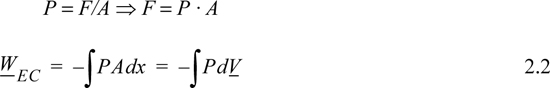
where the subscript EC refers to expansion/contraction work.
In evaluating this expression, a nagging question of perspective comes up. It would be a trivial question except that it causes major headaches when we later try to keep track of positive and negative signs. The question is essentially this: In the discussion above, is positive work being done on the system, or is negative work being done by the system? When we add energy to the system, we consider it a positive input into the system; therefore, putting work into the system should also be considered as a positive input. On the other hand, when a system does work, the energy should go down, and it might be convenient to express work done by the system as positive. The problem is that both perspectives are equally valid—therefore, the choice is arbitrary. Since various textbooks choose differently, there is always confusion about sign conventions. The best we can hope for is to be consistent during our own discussions. We hereby consider work to be positive when performed on the system. Thus, energy put into the system is positive. Because volume decreases when performing work of compression, the sign on the integral for work is negative,

where P and V are of the system. Clarification of “reversible” is given in Section 2.4 on page 42. By comparing Eqn. 2.3 with the definitions of work given by Eqns. 2.1 and 2.2, it should be obvious that the dV term results from expansion/contraction of the boundary of the system. The P results from the force of the system acting at the boundary. Therefore, to use Eqn. 2.3, the pressure in the integral is the pressure of the system at the boundary, and the boundary must move. A system which does not have an expanding/contracting boundary does not have expansion/contraction work.1
2.2. Shaft Work
In a flowing system, we know that a propeller-type device can be used to push a fluid through pipes—this is the basis of a centrifugal pump. Also, a fluid flowing through a similar device could cause movement of a shaft—this is the basis for hydroelectric power generation and the water wheels that powered mills in the early twentieth century. These are the most commonly encountered forms of shaft work in thermodynamics, but there is another slight variation. Suppose an impeller was inserted into a cylinder containing cookie batter and stirred while holding the piston at a fixed volume. We would be putting work into the cylinder, but the system boundaries would neither expand nor contract. All of these cases exemplify shaft work. The essential feature of shaft work is that work is being added or removed without a change in volume of the system. We show in Section 2.8, page 54, that shaft work for a reversible flow process can be computed from

Note that Eqns. 2.3 and 2.4 are distinct and should not be interchanged. Eqn. 2.4 is restricted to shaft work in an open system and Eqn. 2.3 is for expansion/contraction work in a closed system. We later show how selection of the system boundary in a flow system relates the two types of terms on page 54.
2.3. Work Associated with Flow
In engineering applications, most problems involve flowing systems. This means that materials typically flow into a piece of equipment and then flow out of it, crossing well-defined system boundaries in the process. Thus, we need to introduce an additional characterization of work: the work interaction of the system and surroundings when mass crosses a boundary. For example, when a gas is released out of a tank through a valve, the exiting gas pushes the surrounding fluid, doing work on the surroundings. Likewise, when a tank valve is opened to allow gas from a higher pressure source to flow inward, the surroundings do work on the gas already in the system. We calculate the work in these situations most easily by first calculating the rate at which work is done.
Let us first consider a fluid entering a system as shown in Fig. 2.1. We have dW = Fdx, and the work interaction of the system is positive since we are pushing fluid into the system. The rate of work is ![]() , but
, but ![]() is velocity, and F = P·A. Further rearranging, recognizing
is velocity, and F = P·A. Further rearranging, recognizing ![]() , and that the volumetric flow rate may be related to the mass specific volume and the mass flow rate,
, and that the volumetric flow rate may be related to the mass specific volume and the mass flow rate, ![]() ,
,
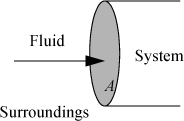
Figure 2.1. Schematic illustration of flow work.
where PV are the properties of the fluid at the point where it crosses the boundary, and ![]() is the absolute value of the mass flow rate across the boundary. When fluid flows out of the system, work is done on the surroundings and the work interaction of the system is
is the absolute value of the mass flow rate across the boundary. When fluid flows out of the system, work is done on the surroundings and the work interaction of the system is
where ![]() is the absolute value of the mass flow across the boundary, and since work is being done on the surroundings, the work interaction of the system is negative. When flow occurs both in and out, the net flow work is the difference:
is the absolute value of the mass flow across the boundary, and since work is being done on the surroundings, the work interaction of the system is negative. When flow occurs both in and out, the net flow work is the difference:
where ![]() and
and ![]() are absolute values of the mass flow rates. For more streams, we simply follow the conventions established, and add inlet streams and subtract outlet streams.
are absolute values of the mass flow rates. For more streams, we simply follow the conventions established, and add inlet streams and subtract outlet streams.
2.4. Lost Work versus Reversibility
In order to properly understand the various characteristic forms that work may assume, we must address an issue which primarily belongs to the upcoming chapter on entropy. The problem is that the generation of disorder reflected by entropy change results in conversion of potentially useful work energy into practically useless thermal energy. If “generation of disorder results in lost work,” then operating in a disorderly fashion results in the lost capability to perform useful work, which we abbreviate by the term: “lost work.” It turns out that the most orderly manner of operating is a hypothetical process known as a reversible process. Typically, this hypothetical, reversible process is applied as an initial approximation of the real process, and then a correction factor is applied to estimate the results for the actual process. It was not mentioned in the discussion of expansion/contraction work, but we implicitly assumed that the process was performed reversibly, so that all of the work on the system was stored in a potentially useful form. To see that this might not always be the case, and how this observation relates to the term “reversible,” consider the problem of stirring cookie batter. Does the cookie batter become unmixed if you stir in the reverse direction? Of course not. The shaft work of stirring has been degraded to effect the randomness of the ingredients. It is impossible to completely recover the work lost in the randomness of this irreversible process. Any real process involves some degree of stirring or mixing, so lost work cannot be eliminated, but we can hope to minimize unnecessary losses if we understand the issue properly.
Consider a process involving gas enclosed in a piston and cylinder. Let the piston be oriented upward so that an expansion of the gas causes the piston to move upward. Suppose that the pressure in the piston is great enough to cause the piston to move upward when the latch is released. How can the process be carried out so that the expansion process yields the maximum work? First, we know that we must eliminate friction to obtain the maximum movement of the piston.
Friction decreases the work available from a process. Frequently we neglect friction to perform a calculation of maximum work.
If we neglect friction, what will happen when we release the latch? The forces are not balanced. Let us take z as our coordinate in the vertical direction, with increasing values in the upward direction. The forces downward on the piston are the force of atmospheric pressure (–Patm · A, where A is the cross-sectional area of the piston) and the force of gravity (–m·g). These forces will be constant throughout movement of the piston. The upward force is the force exerted by the gas (P · A). Since the forces are not balanced, the piston will begin to accelerate upward (F = ma). It will continue to accelerate until the forces become balanced.2 However, when the forces are balanced, the piston will have a non-zero velocity. As it continues to move up, the pressure inside the piston continues to fall, making the upward force due to the inside pressure smaller than the downward force. This causes the piston to decelerate until it eventually stops. However, when it stops at the top of the travel, it is still not in equilibrium because the forces are again not balanced. It begins to move downward. In fact, in the absence of dissipative mechanisms we have set up a perpetual motion.3 A reversible piston would oscillate continuously between the initial state and the state at the top of travel. This would not happen in a real system. One phenomenon which we have failed to consider is viscous dissipation (the effect of viscosity).
Let us consider how velocity gradients dissipate linear motion. Consider two diatomic molecules touching one another which both have exactly the same velocity and are traveling in exactly the same direction. Suppose that neither is rotating. They will continue to travel in this direction at the same velocity until they interact with an external body. Now consider the same two molecules in contact, again moving in exactly the same direction, but one moving slightly faster. Now there is a velocity gradient. Since they are touching one another, the fact that one is moving a little faster than the other causes one to begin to rotate clockwise and the other counter-clockwise because of friction as one tries to move faster than the other. Naturally, the kinetic energy of the molecules will stay constant, but the directional velocities are being converted to rotational (directionless) energies. This is an example of viscous dissipation in a shear situation. In the case of the oscillating piston, the viscous dissipation prevents complete transfer of the internal energy of the gas to the piston during expansion, resulting in a stroke that is shorter than a reversible stroke. During compression, viscous dissipation results in a fixed internal energy rise for a shorter stroke than a reversible process. In both expansion and compression, the temperature of the gas at the end of each stroke is higher than it would be for a reversible stroke, and each stroke becomes successively shorter.
Velocity gradients lead to dissipation of directional motion (kinetic energy) into random motion (internal energy) due to the viscosity of a fluid. Frequently, we neglect viscous dissipation to calculate maximum work. A fluid would need to have zero viscosity for this mechanism of dissipation to be non-existent. Pressure gradients within a viscous fluid lead to velocity gradients; thus, one type of gradient is associated with the other.
We can see that friction and viscosity play an important role in the loss of capability to perform useful work in real systems. In our example, these forces cause the oscillations to decrease somewhat with each cycle until the piston comes to rest. Another possibility of motion that might occur with a piston is interaction with a stop, which limits the travel of the piston. As the piston travels upward, if it hits the stop, it will have kinetic energy which must be absorbed. In a real system, this kinetic energy is converted to internal energy of the piston, cylinder, and gas.
Kinetic energy is dissipated to internal energy when objects collide inelastically, such as when a moving piston strikes a stop. Frequently we imagine systems where the cylinder and piston can neither absorb nor transmit heat; therefore, the lost kinetic energy is returned to the gas as internal energy.
So far, we have identified three dissipative mechanisms. Additional mechanisms are diffusion along a concentration gradient and heat conduction along a temperature gradient, which will be discussed in Chapter 4. Velocity, temperature, and concentration gradients are always associated with losses of work. If we could eliminate them, we could perform maximum work (but it would require infinite time).
A process without dissipative losses is called reversible. A process is reversible if the system may be returned to a prior state by reversing the motion. We can usually determine that a system is not reversible by recognizing when dissipative mechanisms exist.
Approaching Reversibility
We can approach reversibility by eliminating gradients within our system. To do this, we can perform motion by differential changes in forces, concentrations, temperatures, and so on. Let us consider a piston with a weight on top, at equilibrium. If we slide the weight off to the side, the change in potential energy of the weight is zero, and the piston rises, so its potential energy increases. If the piston hits a stop, kinetic energy is dissipated. Now let us subdivide the weight into two portions. If we move off one-half of the weight, the piston strikes the stop with less kinetic energy than before, and in addition, we have now raised half of the weight. If we repeat the subdivision again we would find that we could move increasing amounts of weight by decreasing the weight we initially move off the piston. In the limit, our weight would become like a pile of sand, and we would remove one grain at a time. Since the changes in the system are so small, only infinitesimal gradients would ever develop, and we would approach reversibility. The piston would never develop kinetic energy which would need to be dissipated.
Reversibility by a Series of Equilibrium States
When we move a system differentially, as just discussed, the system is at equilibrium along each step of the process. To test whether the system is at equilibrium at a particular stage, we can imagine freezing the process at that stage. Then we can ask whether the system would change if we left it at those conditions. If the system would remain static (i.e., not changing) at those conditions, then it must be at equilibrium. Because it is static, we could just as easily go one way as another ⇒ “reversible.” Thus, reversible processes are the result of infinitesimal driving forces.
Reversibility by Neglecting Viscosity and Friction
Real processes are not done infinitely slowly. In the previous examples we have used idealized pistons and cylinders for discussion. Real systems can be far from ideal and may have much more complex geometry. For example, projectiles can be fired using gases to drive them, and we need a method to estimate the velocities with which they are projected into free flight. One application of this is the steam catapult used to assist airplanes in becoming airborne from the short flight decks of aircraft carriers. Another application would be determination of the exit velocity of a bullet fired from a gun. These are definitely not equilibrium processes, so how can we begin to calculate the exit velocities? Another case would be the centrifugal pump. The pump works by rapidly rotating a propeller-type device. The pump simply would not work at low speed without velocity gradients! So what do we do in these cases? The answer is that we perform a calculation ignoring viscosity and friction. Then we apply an efficiency factor to calculate the real work done. The efficiency factors are determined empirically from our experience with real systems of a similar nature to the problem at hand. Efficiencies are introduced in Chapter 4. In the remainder of this chapter, we concentrate on the first part of the problem, calculation of reversible work.
![]() Viscosity and friction are frequently ignored for an estimation of optimum work, and an empirical efficiency factor is applied based on experience with similar systems.
Viscosity and friction are frequently ignored for an estimation of optimum work, and an empirical efficiency factor is applied based on experience with similar systems.
Example 2.1. Isothermal reversible compression of an ideal gas
Calculate the work necessary to isothermally perform steady compression of two moles of an ideal gas from 1 to 10 bar and 311 K in a piston. An isothermal process is one at constant temperature. The steady compression of the gas should be performed such that the pressure of the system is always practically equal to the external pressure on the system. We refer to this type of compression as “reversible” compression.
Solution
System: closed; Basis: one mole

WEC = –8.314 J/mol-K · 311 K ln(1/10) = 5954 J/mol
WEC = 2(5954) = 11,908 J
Note: Work is done on the gas since the sign is positive. This is the sign convention set forth in Eqn. 2.3. If the integral for Eqn. 2.3 is always written as shown with the initial state as the lower limit of integration and the P and V properties of the system, the work on the gas will always result with the correct sign.
2.5. Heat Flow
A very simple experiment shows us that heat transport is also related to energy. If two steel blocks of different temperature are placed in contact with one another, but otherwise are insulated from their surroundings, they will come to equilibrium at a common intermediate temperature. The warmer block will be cooled, and the colder block will be warmed.
Qblock 1 = –Qblock 2
Heat is transferred at a boundary between the blocks. Therefore, heat is not a property of the system. It is a form of interaction at the boundary which transfers internal energy. If heat is added to a system for a finite period of time, then the energy of the system increases because the kinetic energy of the molecules is increased. When an object feels hot to our touch, it is because the kinetic energy of molecules is readily transferred to our hand.
Since the rate of heating may vary with time, we must recognize that the total heat flows must be summed (or integrated) over time. In general, we can represent a differential contribution by
We can also relate the internal energy change and heat transfer for either block in a differential form:
An idealized system boundary that has no resistance to heat transfer but is impervious to mass is called a diathermal wall.
2.6. Path Properties and State Properties
In the previous example, we have used an isothermal path. It is convenient to define other terms which describe pathways concisely. An isobaric path is one at constant pressure. An isochoric path is one at constant volume. An adiabatic path is one without heat transfer.
The heat and work transfer necessary for a change in state are dependent on the pathway taken between the initial and final states. A state property is one that is independent of the pathway taken. For example, when the pressure and temperature of a gas are changed and the gas is returned to its initial state, the net change in temperature, pressure, and internal energy is zero, and these properties are therefore state properties. However, the net work and net heat transfer will not necessarily be zero; their values will depend on the path taken. Also, it is helpful to recall that heat and work are not properties of the system; therefore, they are not state properties.
![]() The work and heat transfer necessary for a change in state are dependent on the pathway taken between the initial and final state.
The work and heat transfer necessary for a change in state are dependent on the pathway taken between the initial and final state.
Example 2.2. Work as a path function
Consider 1.2 moles of an ideal gas in a piston at 298 K and 0.2 MPa and at volume V1. The gas is expanded isothermally to twice its original volume, then cooled isobarically to V1. It is then heated at constant volume back to T1. Demonstrate that the net work is non-zero, and that the work depends on the path.
First sketch the process on a diagram to visualize the process as shown in Fig. 2.2. Determine the initial volume:
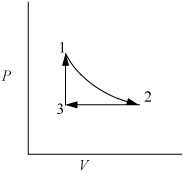
Figure 2.2. Schematic for Example 2.2.

1. Isothermally expand that gas:

2. Isobarically cool down to V1:
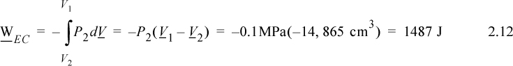
3. Heat at constant volume back to T1:
⇒WEC = 0 (because dV = 0 over entire step)
We have returned the system to its original state and all state properties have returned to their initial values. What is the total work done on the system?
Therefore, we conclude that work is a path function, not a state function.
Exercise: If we reverse the path, the work will be different; in fact, it will be positive instead of negative (+573.6 J). If we change the path to isobarically expand the gas to double the volume (W = –2973 J), cool to T1 at constant volume (W = 0 J), then isothermally compress to the original volume (W = –2060 J), the work will be –913 J.
Note: Heat was added and removed during the process of Example 2.2 which has not been accounted for above. The above process transforms work into heat, and all we have done is computed the amount of work. The amount of heat is obviously equal in magnitude and opposite in sign, in accordance with the first law. The important thing to remember is that work is a path function, not a state function.
2.7. The Closed-System Energy Balance
A closed system is one in which no mass flows in or out of the system, as shown in Fig. 2.3. The introductory sections have discussed heat and work interactions, but we have not yet coupled these to the energy of the system. In the transformations we have discussed, energy can cross a boundary in the form of expansion/contraction work (–∫ PdV), shaft work (WS), and heat (Q)4. There are only two ways a closed system can interact with the surroundings, via heat and work interactions. If we put both of these possibilities into one balance equation, then developing the balance for a given application is simply a matter of analyzing a given situation and deleting the balance terms that do not apply. The equation terms can be thought of as a check list.
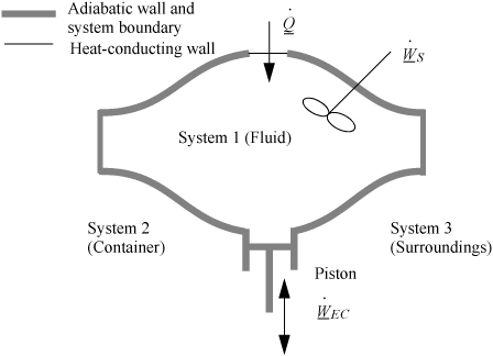
Figure 2.3. Schematic of a closed system.
Experimentally, scientists discovered that if heat and work are measured for a cyclical process which returns to the initial state, the heat and work interactions together always sum to zero. This is an important result! This means that, in non-cyclical processes where the sum of heat and work is non-zero, the system has stored or released energy, depending on whether the sum is positive or negative. In fact, by performing enough experiments, scientists decided that the sum of heat and work interactions in a closed system is the change in energy of the system! To develop the closed-system energy balance, let us first express the balance in terms of words.
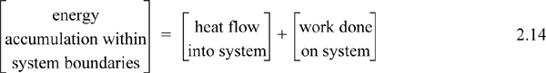
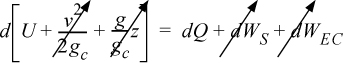
Energy within the system is composed of the internal energy (e.g., U), and the kinetic (mu2/2gc) and potential energy (mgz/gc) of the center of mass. For closed systems, the “check list” equation is:

The left-hand side summarizes changes occurring within the system boundaries and the right-hand side summarizes changes due to interactions at the boundaries. It is a recommended practice to always write the balance in this convention when starting a problem. We will follow this convention throughout example problems in Chapters 2–4 and relax the practice subsequently. The kinetic and potential energy of interest in Eqn. 2.15 is for the center of mass, not the random kinetic and potential energy of molecules about the center of mass. The balance could also be expressed in terms of molar quantities, but if we do so, we need to introduce molecular weight in the potential and kinetic energy terms. Since the mass is constant in a closed system, we may divide the above equation by m,

![]() Closed-system balance. The left-hand side summarizes changes inside the boundaries, and the right-hand side summarizes interactions at the boundaries.
Closed-system balance. The left-hand side summarizes changes inside the boundaries, and the right-hand side summarizes interactions at the boundaries.
where heat and work interactions are summed for multiple interactions at the boundaries. We can integrate Eqn. 2.16 to obtain
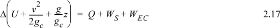
We may also express the energy balance in terms of rates of change,
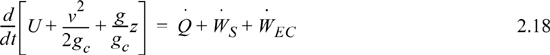
where ![]() ,
, ![]() and
and ![]() Frequently, the kinetic and potential energy changes are small (as we will show in Example 2.9), in a closed system shaft work is not common, and the balance simplifies to
Frequently, the kinetic and potential energy changes are small (as we will show in Example 2.9), in a closed system shaft work is not common, and the balance simplifies to

Example 2.3. Internal energy and heat
In Section 2.5 on page 46 we discussed that heat flow is related to the energy of system, and now we have a relation to quantify changes in energy. If 2000 J of heat are passed from the hot block to the cold block, how much has the internal energy of each block changed?
Solution
First choose a system boundary. Let us initially place system boundaries around each of the blocks. Let the warm block be block1 and the cold block be block2. Next, eliminate terms which are zero or are not important. The problem statement says nothing about changes in position or velocity of the blocks, so these terms can be eliminated from the balance. There is no shaft involved, so shaft work can be eliminated. The problem statement doesn’t specify the pressure, so it is common to assume that the process is at a constant atmospheric pressure of 0.101 MPa. The cold block does expand slightly when it is warmed, and the warm block will contract; however, since we are dealing with solids, the work interaction is so small that it can be neglected. For example, the blocks together would have to change 10 cm3 at 0.101 MPa to equal 1 J out of the 2000 J that are transferred.
Therefore, the energy balance for each block becomes:
We can integrate the energy balance for each block:
The magnitude of the heat transfer between the blocks is the same since no heat is transferred to the surroundings, but how about the signs? Let’s explore that further. Now, placing the system boundary around both blocks, the energy balance becomes:
Note that the composite system is an isolated system since all heat and work interactions across the boundary are negligible. Therefore, ΔU = 0 or by dividing in subsystems, ΔUblock1 + ΔUblock2 = 0 which becomes ΔUblock1 = –ΔUblock2. Notice that the signs are important in keeping track of which system is giving up heat and which system is gaining heat. In this example, it would be easy to keep track, but other problems will be more complicated, and it is best to develop a good bookkeeping practice of watching the signs. In this example the heat transfer for the initially hot system will be negative, and the heat transfer for the other system will be positive. Therefore, the internal energy changes are ΔUblock1 = –2000 J and ΔUblock2 = 2000 J.
Although very simple, this example has illustrated several important points.
1. Before simplifying the energy balance, the boundary should be clearly described by a statement and/or a sketch.
2. A system can be subdivided into subsystems. The composite system above is isolated, but the subsystems are not. Many times, problems are more easily solved, or insight is gained by looking at the overall system. If the subsystem balances look difficult to solve, try an overall balance.
3. Positive and negative energy signs are important to use carefully.
4. Simplifications can be made when some terms are small relative to other terms. Calculation of the expansion contraction work for the solids is certainly possible above, but it has a negligible contribution. However, if the two subsystems had included gases, then this simplification would have not been reasonable.
2.8. The Open-System, Steady-State Balance
Having established the energy balance for a closed system, and, from Section 2.3, the work associated with flowing fluids, let us extend these concepts to develop the energy balance for a steady-state flow system. The term steady-state means the following:
1. All state properties throughout the system are invariant with respect to time. The properties may vary with respect to position within the system.
2. The system has constant mass, that is, the total inlet mass flow rate equals the total outlet mass flow rates, and all flow rates are invariant with respect to time.
3. The center of mass for the system is fixed in space. (This restriction is not strictly required, but will be used throughout this text.)
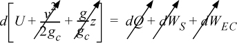
To begin, we write the balance in words, by adding flow to our previous closed-system balance. There are only three ways the surroundings can interact with the system: flow, heat, and work. A schematic of an open steady-state system is shown in Fig. 2.4. In consideration of the types of work encountered in steady-state flow, recognize that expansion/contraction work is rarely involved, so this term is omitted at this preliminary stage. This is because we typically apply the steady-state balance to systems of rigid mechanical equipment, and there is no change in the size of the system. Therefore, the expansion/contraction work term is set to 0.
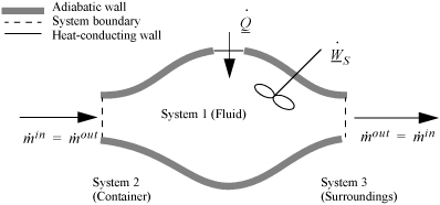
Figure 2.4. Schematic of a steady-state flow system.
The balance in words becomes time-dependent since we work with flow rates:
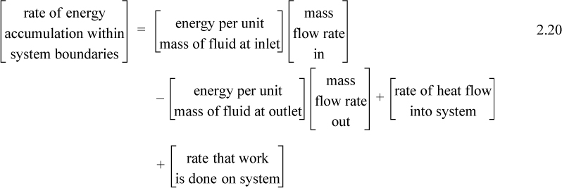
Again, we follow the convention that the left-hand side quantifies changes inside our system. Consider the change of energy inside the system boundary given by the left-hand side of the equation. Due to the restrictions placed on the system by steady-state, there is no accumulation of energy within the system boundaries, so the left-hand side of Eqn. 2.20 becomes 0.
As a result,

where heat and work interactions are summed over all boundaries. The flow work from Eqn. 2.7 may be inserted and summed over all inlets and outlets,
and combining flow terms:

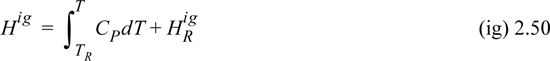
Enthalpy
Note that the quantity (U + PV) arises quite naturally in the analysis of flow systems. Flow systems are very common, so it makes sense to define a single symbol that denotes this quantity:
H ≡ U + PV
Thus, we can tabulate precalculated values of H and save steps in calculations for flow systems. We call H the enthalpy.
The open-system, steady-state balance is then,
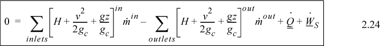
where the heat and work interactions are summations of the individual heat and work interactions over all boundaries.
Note: Q is positive when the system gains heat energy; W is positive when the system gains work energy; ![]() and
and ![]() are always positive; and
are always positive; and ![]() is positive when the systems gains mass and zero for steady-state flow. Mass may be replaced with moles in a non-reactive system with appropriate care for unit conversion.
is positive when the systems gains mass and zero for steady-state flow. Mass may be replaced with moles in a non-reactive system with appropriate care for unit conversion.
Note that the relevant potential and kinetic energies are for the fluid entering and leaving the boundaries, not for the fluid which is inside the system boundaries. When only one inlet and one outlet stream are involved, the steady-state flow rates must be equal, and

When kinetic and potential energy changes are negligible, we may write

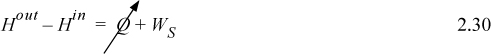
where ΔH = Hout – Hin. We could use molar flow rates for Eqns. 2.24 through 2.26 with the usual care for unit conversions of kinetic and potential energy. For an open steady-state system meeting the restrictions of Eqn. 2.26, we may divide through by the mass flow rate to find
In common usage, it is traditional to relax the convention of keeping only system properties on the left side of the equation. More simply we often write:
Compare Eqns. 2.19 and 2.28. Energy and enthalpy do not come from different energy balances, where the “closed system” balance uses U and WEC and the “open system” balance uses H and Ws. Rather, the terms result from logically simplifying the generalized energy balance shown in the next section.
Comment on Δ Notation
In a closed system we use the Δ symbol to denote the change of a property from initial state to final state. In an open, steady-state system, the left-hand side of the energy balance is zero. Therefore, we frequently write Δ as a shorthand notation to combine the first two flow terms on the right-hand side of the balance, with the symbol meaning “outlet relative to inlet” as shown above. You need to learn to recognize which terms of the energy balance are zero or insignificant for a particular problem, whether a solution is for a closed or open system, and whether the Δ symbol denotes “outlet relative to inlet” or “final relative to initial.”
Understanding Enthalpy and Shaft Work
Consider steady-state, adiabatic, horizontal operation of a pump, turbine, or compressor. It is possible to conceive of a closed packet of fluid as the system while it flows through the equipment. After analyzing the system from this perspective, we can switch to the open-system perspective to gain insight about the relation between open systems and closed systems, energy and enthalpy, and EC work and shaft work. As a bonus, we obtain a handy relation for estimating pump work and the enthalpy of compressed liquids.
In the conception of a closed-system fluid packet, no mass moves across the system boundary. The system, as we have chosen it, does not include a shaft even though it will move past the shaft. If you have trouble seeing this, remember that the system boundaries are defined by the conceived packet of mass. Since the system boundary does not contain the shaft before the packet enters, or after the packet exits, it cannot contain the shaft as it moves through the turbine. The system simply deforms to envelope the shaft. Therefore, all work for this closed system is technically expansion/contraction work; the closed-system expansion/contraction work is composed of the flow work and shaft work that we have seen from the open-system perspective. It is difficult to describe exactly what happens to the system at every point, but we can say something about how it begins and how it ends. This observation leads to what is called an integral method of analysis.
System: closed, adiabatic; Basis: packet of mass m. The kinetic and potential energy changes are negligible:
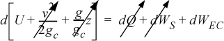
Integrating from the inlet (initial) state to the outlet (final) state:
Uout – Uin = WEC
We may change the form of the integral representing work via integration by parts:
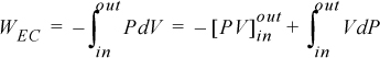
We recognize the term PV as representing the work done by the flowing fluid entering and leaving the system; it does not contribute to the work of the device. Therefore, the work interaction with the turbine is the remaining integral, ![]() . Substitution gives,
. Substitution gives,

Switching to the open-system perspective, Eqn. 2.28 gives
Recalling that H = U + PV and comparing the last two equations means Ws = ∫VdP is the work done using the pump, compressor, or turbine as the system. Furthermore, the appearance of the PV contribution in combination with U occurs naturally as part of the integration by parts. Physically, work is always “force times distance.” Though this derivation has been restricted to an adiabatic device, the result is general to devices including heat transfer as we show later in Section 5.7.

Note: The shaft work given by dWS = VdP is distinct from expansion/contraction work, dWEC = PdV. Moreover, both are distinct from flow work, dWflow = PVdm.
Several practical issues may be considered in light of Eqn. 2.31. First, the work done on the system is negative when the pressure change is negative, as in proceeding through a turbine or expander. This is consistent with our sign convention. Second, when considering gas flow, the integration may seem daunting if an ideal gas is not involved because of the complicated manner that V changes with T and P. Rather, for gases, we can frequently work with the enthalpy for a given state change. The enthalpy values for a state change read from a table or chart lead to Ws directly using Eqn. 2.30. For liquids, however, the integral can be evaluated quickly. Volume can often be approximated as constant, especially when Tr < 0.75. In that case, we obtain by integration an equation for estimating pump work:
![]() Shaft work for a liquid pump or turbine where kinetic and potential energy changes are small and Tr < 0.75 so that the fluid is incompressible.
Shaft work for a liquid pump or turbine where kinetic and potential energy changes are small and Tr < 0.75 so that the fluid is incompressible.
Example 2.4. Pump work for compressing H2O
Use Eqn. 2.31 to estimate the work of compressing 20°C H2O from a saturated liquid to 5 and 50 MPa. Compare to the values obtained using the compressed liquid steam tables.
Solution
For H2O, Tr = 0.75 corresponds to 212°C, so we are safe on that count. We can calculate the pump work from Eqn. 2.31, reading Psat = 0.00234 MPa and VL = 1.002 cm3/g from the saturation tables at 20°C:
⇒ ΔH ≈ VLΔP = 1.002 cm3/g(50 MPa – 0.00234 MPa) = 50.1 MPa-cm3/g for 50 MPa
⇒ ΔH ≈ VLΔP = 1.002 cm3/g(100 MPa – 0.00234 MPa) = 100.2 MPa-cm3/g for 100 MPa
A convenient way of converting units for these calculations is to multiply and divide by the gas constant, noting its different units. This shortcut is especially convenient in this case, e.g.,
ΔH = 50.1 MPa-cm3/g ·(8.314 J/mole-K)/(8.314 MPa-cm3/mole-K) = 50.1 kJ/kg
ΔH = 100.2 MPa-cm3/g ·(8.314 J/mole-K)/(8.314 MPa-cm3/mole-K) = 100.2 kJ/kg
Note that, for water, the change in enthalpy in kJ/kg is roughly equal to the pressure rise in MPa because the specific volume is so close to one and Psat << P. That is really handy.
The saturation enthalpy is read from the saturation tables as 83.95 kJ/kg. The values given in the compressed liquid table (at the end of the steam tables) are 88.6 kJ/kg at 5 MPa and 130 kJ/kg at 50 MPa, corresponding to estimated work values of 4.65 and 46.1 kJ/kg. The estimation error in the computed work is about 7 to 9%, and smaller for lower pressures. This degree of precision is generally satisfactory because the pump work itself is usually small relative to other work and terms (like the work produced by a turbine in a power cycle).
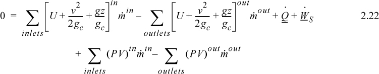
2.9. The Complete Energy Balance
An open-system that does not meet the requirements of a steady-state system is called an unsteady-state open-system as shown in Fig. 2.5. The mass-in may not equal the mass-out, or the system state variables (e.g., temperature) may change with time, so the system itself may gain in internal energy, kinetic energy, or potential energy. An example of this is the filling of a tank being heated with a steam jacket. Another example is the inflation of a balloon, where there is mass flow in and the system boundary expands. These considerations lead to a general equation which is applicable to open or closed systems,

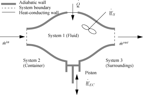
Figure 2.5. Schematic of a general system.
where the heat and work interactions are summations of the individual heat and work interactions over all boundaries. We also may write this with the time dependence implied:
Note: The signs and conventions are the same as presented following Eqn. 2.24.
Usually, the closed-system or the steady-state equations are sufficient by themselves. But for unsteady-state open systems, the entire equation must be considered. Fortunately, even when the entire energy balance is applied, some of the terms are usually not necessary for a given problem, so fewer terms are usually needed than shown in Eqn. 2.33. An objective of this text is to build your ability to recognize which terms apply to a given problem.
2.10. Internal Energy, Enthalpy, and Heat Capacities
Before we proceed with more examples, we need to add another thermodynamic tool. Unfortunately, there are no “internal energy” or “enthalpy” meters. In fact, these state properties must be “measured” indirectly by other state properties. The Gibbs phase rule tells us that if two state variables are fixed in a pure single-phase system, then all other state variables will be fixed. Therefore, it makes sense to measure these properties in terms of P, V, and T. In addition, if this relation is developed, it will enable us to find P, V, and/or T changes for a given change in ΔU or ΔH. In Example 2.3, where a warm and cold steel blocks were contacted, we solved the problem without calculating the change in temperature for each block. However, if we had a relation between U and T, we could have calculated the temperature changes. The relations that we seek are the definitions of the heat capacities.
Constant Volume Heat Capacity
The constant of proportionality between the internal energy change at constant volume and the temperature change is known as the constant volume heat capacity. The constant volume heat capacity is defined by:
Since temperature changes are easily measured, internal energy changes can be calculated once CV is known. CV is not commonly tabulated, but, as shown below, it can be easily determined from the constant pressure heat capacity, which is commonly available.
Constant Pressure Heat Capacity
In the last two sections, we have introduced enthalpy, and we can relate the change in enthalpy of a system to temperature in a manner analogous to the method used for internal energy. This relationship will involve a new heat capacity, the heat capacity at constant pressure defined by:
where H is the enthalpy of the system.
The use of two heat capacities, CV and CP, forces us to think of constant volume or constant pressure as the important distinction between these two quantities. The important quantities are really internal energy versus enthalpy. You simply must convince yourself to remember that CV refers to changes in U at constant volume, and CP refers to changes in H at constant pressure.
Relations between Heat Capacities, U and H
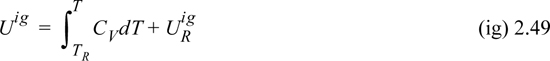
We have said that CV values are not readily available; therefore, how do we determine internal energy changes? Also, how do we determine enthalpy changes at constant volume or internal energy changes at constant pressure? We will return to the details of these questions in Chapters 6–8 and handle them rigorously, but the details have been rigorously followed by developers of thermodynamic charts and tables. Therefore, for relating the internal energy or enthalpy to temperature and pressure, a thermodynamic chart or table is preferred. If none is available, or properties are not tabulated in the state of interest, some exact relations and some approximate rules of thumb must be applied. The relations are also useful for introductory calculations while focus is on the energy balance rather than the property relations.
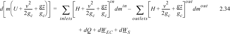
For an ideal gas,
Constant pressure heat capacities for ideal gases are tabulated in Appendix E. Constant volume heat capacities for ideal gases can readily be determined from Eqn. 2.38. For ideal gases, internal energy and enthalpy are independent of pressure as we implied with Eqn. 1.21. For real gases and for liquids, the relation between CP and CV is more complex, and derivatives of P-V-T properties must be used as shown rigorously in Examples 6.1, 6.6, and 6.9 and implemented thereafter. We will use thermodynamic tables and charts for real gases until these relations are developed.
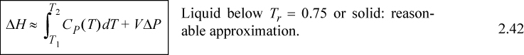
For liquids or solids, we typically calculate ΔH and correct the calculation if necessary as explained below. For liquids, it has been experimentally determined that internal energy is only very weakly dependent on pressure below Tr = 0.75. In addition, the molar volume is insensitive to pressure below Tr = 0.75. We demonstrated in Example 2.4 that,
![]() is the reduced temperature calculated by dividing the absolute temperature by the critical temperature. (A rigorous evaluation is considered in Example 6.1 on page 233.) The relations for solids and liquids are important because frequently the properties have not been measured, or the measurements available in charts and tables are not available at the pressures of interest. We may then summarize the relations of internal energy and enthalpy with temperature.
is the reduced temperature calculated by dividing the absolute temperature by the critical temperature. (A rigorous evaluation is considered in Example 6.1 on page 233.) The relations for solids and liquids are important because frequently the properties have not been measured, or the measurements available in charts and tables are not available at the pressures of interest. We may then summarize the relations of internal energy and enthalpy with temperature.

Note: These formulas do not account for phase changes which may occur.
Note that the heat capacity of a monatomic ideal gas can be obtained by differentiating the internal energy as given in Chapter 1, resulting in CV = 3/2 R and CP = 5/2 R. Heat capacities for diatomics are larger, CP = 7/2 R, and CV = 5/2 R near room temperature, and polyatomics are larger still. According to classical theory, each degree of freedom5 contributes 1/2R to CV. Kinetic and potential energy each contribute a degree of freedom in each dimension. A monatomic ideal gas has only three kinetic energy degrees of freedom, thus CV = 3/2 R. Diatomic molecules are linear so they have two additional degrees of freedom for the linear (one-dimensional) bond that has kinetic and potential energy both. In complicated molecules, the vibrations are characterized by modes. See the endflap to make a quick comparison. Monatomic solids have three degrees of freedom each for kinetic and vibrational energy, one for each principle direction, thus the law of Dulong and Petit, CVS = 3R is a first approximation. Low-temperature heat capacities of monatomic solids are explored more in Example 6.8. If you become curious about the manner in which the heat capacities of polyatomic species differ from those of the spherical molecules discussed in Chapter 1, you will find introductions to statistical thermodynamics explain the contributions of translation, rotation, and vibration. For polyatomic molecules, the heat capacity increases with molecular weight due to the increased number of degrees of freedom for each bond. In this text, ideal gas heat capacity values at 298 K are summarized inside the back cover of the book, and may be assumed to be independent of temperature over small temperature ranges near room temperature. The increase in heat capacity with temperature for diatomics and polyatomics is dominated by the vibrational contribution. The treatment of heat capacity by statistical thermodynamics is particularly interesting because it is a theory6 that often gives more accurate results than experimental calorimetric measurements. Commonly, engineers correlate ideal gas heat capacities with expressions like polynomials.
![]() Whenever we assume heat capacity to be temperature independent in this text, we mark the equation with a (*) symbol near the right margin.
Whenever we assume heat capacity to be temperature independent in this text, we mark the equation with a (*) symbol near the right margin.
We will frequently ignore the heat capacity dependence on T to make an approximate calculation. Whenever we assume heat capacity to be temperature independent in this text, we mark the equation with a (*) symbol near the right margin. Heat capacities represented as polynomials of temperature are available in Appendix E. The heat capacity depends on the state of aggregation. For example, water has a different heat capacity when solid (ice), liquid, or vapor (steam). The contribution of the heat capacity integral to the energy balance is frequently termed the sensible heat to communicate its contribution relative to latent heat (due to phase changes) or heat of reaction to be discussed later. Note that these are called “heats” even though they are enthalpy changes.
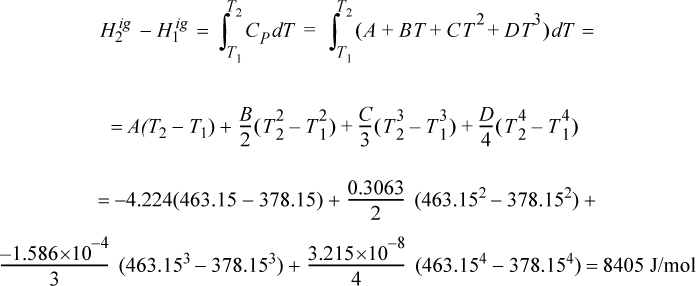
Example 2.5. Enthalpy change of an ideal gas: Integrating CPig(T)
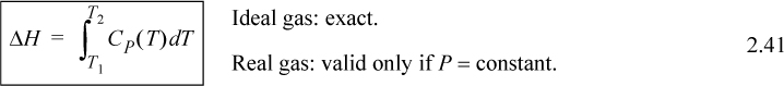
Propane gas undergoes a change of state from an initial condition of 5 bar and 105°C to 25 bar and 190°C. Compute the change in enthalpy using the ideal gas law.
Solution
The ideal gas change is calculated via Eqn. 2.41 and is independent of pressure. The heat capacity constants are obtained from Appendix E.
Example 2.6. Enthalpy of compressed liquid
The compressed liquid tables are awkward to use for compressed liquid enthalpies because the pressure intervals are large. Using saturated liquid enthalpy values for water and hand calculations, estimate the enthalpy of liquid water at 20°C H2O and 5 and 50 MPa. Compare to the values obtained using the compressed liquid steam tables.
Solution
This is a common calculation needed for working with power plant condensate streams at high pressure. The relevant equation is Eqn. 2.42, but we can eliminate the temperature integral by selecting saturated water at the same temperature and then applying the pressure correction, i.e., applying Eqn. 2.39, ΔH ≈ VΔP relative to the saturation condition, giving H = Hsat + VΔP. The numerical calculations have already been done in Example 2.4 on page 55. Both calculations use the same approximation, even though the paths are slightly different. A more rigorous analysis is shown later in Example 6.1.
![]() This is a common calculation needed for working with power plant condensate streams at high pressure.
This is a common calculation needed for working with power plant condensate streams at high pressure.
Example 2.7. Adiabatic compression of an ideal gas in a piston/cylinder
Nitrogen is contained in a cylinder and is compressed adiabatically. The temperature rises from 25°C to 225°C. How much work is performed? Assume that the heat capacity is constant (CP/R = 7/2), and that nitrogen follows the ideal gas law.
Solution
System is the gas. Closed system, system size changes, adiabatic.

Note that because the temperature rise is specified, we do not need to know if the process was reversible.
Relation to Property Tables/Charts
In Section 1.4, we used steam tables to find internal energies of water as liquid or vapor. Tables or charts usually contain enthalpy and internal energy information, which means that these properties can be read from the source for these compounds, eliminating the need to apply Eqns. 2.40–2.43. This is usually more accurate because the pressure dependence of the properties that Eqns. 2.40–2.43 neglect has been included in the table/chart, although the pressure correction method applied in the previous example for liquids is generally accurate enough for liquids. Energy and enthalpy changes spanning phase transitions can be determined directly from the tables since energies and enthalpies of phase transitions are implicitly included in tabulated values.
Estimation of Heat Capacities
If heat capacity information cannot be located from appendices in this text, from the NIST Chemistry WebBook7, or from reference handbooks, it can be estimated by several techniques offered in the Chemical Engineer’s Handbook8 and The Properties of Gases and Liquids.9
Phase Transitions (Liquid-Vapor)
Enthalpies of vaporization are tabulated in Appendix E for selected substances at their normal boiling temperatures (their saturation temperatures at 1.01325 bar). In the case of the steam tables, Section 1.4 shows that the energies and enthalpies of vaporization of water are available along the entire saturation curve. Complete property tables for some other compounds are available in the literature or online, however, most textbooks present charts to conserve space, and we follow that trend. In the cases where tables or charts are available, their use is preferred for phase transitions away from the normal boiling point, although a hypothetical path that passes through the normal boiling point can usually be constructed easily.
The energy of vaporization is more difficult to find than the enthalpy of vaporization. It can be calculated from the enthalpy of vaporization and the P-V-T properties. Since U = H – PV,
ΔUvap = ΔHvap – Δ(PV)vap = ΔHvap – (PsatV)V – (PsatV)L = ΔHvap – Psat(VV – VL)
Far from the critical point, the molar volume of the vapor is much larger than the molar volume of the liquid. Further, at the normal boiling point (the saturation temperature at 1.01325 bar), the ideal gas law is often a good approximation for the vapor volume,
Estimation of Enthalpies of Vaporization
If the enthalpy of vaporization cannot be located in the appendices or a standard reference book, it may be estimated by several techniques offered and reviewed in the Chemical Engineer’s Handbook and The Properties of Gases and Liquids. One particularly convenient correlation is10

where Tr is reduced temperature, ω is the acentric factor (to be described in Chapter 7), also available on the back flap. If accurate vapor pressures are available, the enthalpy of vaporization can be estimated far from the critical point (i.e., Tr < 0.75) by the Clausius–Clapeyron equation:

The background for this equation is developed in Section 9.2. Vapor pressure is often represented by the Antoine equation, logPsat = A – B/(T + C). If Antoine parameters are available, they may be used to estimate the derivative term of Eqn. 2.46,

where T is in °C, and B and C are Antoine parameters for the common logarithm of pressure. For Antoine parameters intended for other temperature or pressure units, the equation must be carefully converted. The temperature limits for the Antoine parameters must be carefully followed because the Antoine equation does not extrapolate well outside the temperature range where the constants have been fit. If Antoine parameters are unavailable, they can be estimated to roughly 10% accuracy by the shortcut vapor pressure (SCVP) model, discussed in Section 9.3,
where the units of Pc match the units of Psat, Tc is in K, and T is in °C.
Phase Transitions (Solid-Liquid)
Enthalpies of fusion (melting) are tabulated for many substances at the normal melting temperatures in the appendices as well as handbooks. Internal energies of fusion are not usually available, however the volume change on melting is usually very small, resulting in internal energy changes that are nearly equal to the enthalpy changes:
Unlike the liquid-vapor transitions, where Tsat depends on pressure, the melting (solid-liquid) transition temperature is almost independent of pressure, as illustrated schematically in Fig. 1.7.
2.11. Reference States
Notice that our heat capacities do not permit us to calculate absolute values of internal energy or enthalpy; they simply permit us to calculate changes in these properties. Therefore, when is internal energy or enthalpy equal to zero—at a temperature of absolute zero? Is absolute zero a reasonable place to assign a reference state from which to calculate internal energies and enthalpies? Actually, we don’t usually solve this problem in engineering thermodynamics for the following two reasons:11 1) for a gas, there would almost always be at least two phase transitions between room temperature and absolute zero that would require knowledge of energy changes of phase transitions and heat capacities of each phase; and 2) even if phase transitions did not occur, the empirical fit of the heat capacity represented by the constants in the appendices are not valid down to absolute zero! Therefore, for engineering calculations, we arbitrarily set enthalpy or internal energy equal to zero at some convenient reference state where the heat capacity formula is valid. We calculate changes relative to this state. The actual enthalpy or internal energy is certainly not zero, it just makes our reference state location clear. If we choose to set the value of enthalpy to zero at the reference state, then HR = 0, and UR = HR – (PV)R where we use subscript R to denote the reference state. Note that UR and HR cannot be precisely zero simultaneously at the reference state. The reference state for water (in the steam tables) is chosen to set enthalpy of water equal to zero at the triple point. Note that PV is negligible at the reference state so that it appears that UR is also zero to the precision of the tabulated values, which is not rigorously correct. (Can you verify this in the steam tables? Which property is set to zero, and for which state of aggregation?). To clearly specify a reference state we must specify:
1. The composition which may or may not be pure.
2. The state of aggregation (S, L, or V).
3. The pressure.
4. The temperature.
As you will notice in the following problems, reference states are not necessary when working with a pure fluid in a closed system or in a steady-state flow system with a single stream. The numerical values of the changes in internal energy or enthalpy will be independent of the reference state.
![]() Reference states are not required for steady-state flow systems with only a few streams, but are recommended when many streams are present.
Reference states are not required for steady-state flow systems with only a few streams, but are recommended when many streams are present.
When multiple components are involved, or many inlet/outlet streams are involved, definition of reference states is recommended since flow rates of the inlet and outlet streams will not necessarily match one-to-one. The reference state for each component may be different, so the reference temperature, pressure, and state of aggregation must be clearly designated.
For unsteady-state open systems that accumulate or lose mass, reference states are imperative when values of ΔU or ΔH changes of the system or surroundings are calculated as the numerical values depend on the reference state. It is only when the changes for the system and surroundings are summed together that the reference state drops out for unsteady-state open systems.
Ideal Gas Properties
For an ideal gas, we must specify only the reference T and P.12 An ideal gas cannot exist as a liquid or solid, and this fact completely specifies the state of our system. In addition, we need to set HR or UR (but not both!) equal to zero.
Also at all states, including the reference state, ![]() . The ideal gas approximation is reliable when contributions from intermolecular potential energy are relatively small. A convenient guideline is, in term of reduced temperature Tr = T/Tc, and reduced pressure Pr = P/Pc, where Pc is the critcal pressure.
. The ideal gas approximation is reliable when contributions from intermolecular potential energy are relatively small. A convenient guideline is, in term of reduced temperature Tr = T/Tc, and reduced pressure Pr = P/Pc, where Pc is the critcal pressure.
State Properties Including Phase Changes
Problems will often involve phase changes. Throughout a problem, since the thermodynamic properties must always refer to the same reference state, phase changes must be incorporated into state properties relative to the state of aggregation of the reference state. To calculate a property for a fluid at T and P relative to a reference state in another phase, a sketch of the pathway from the reference state is helpful to be sure all steps are included. Several pathways are shown in Fig. 2.6 for different reference states. Note that the ideal gas reference state with the generalized correlation for the heat of vaporization (option (c)) is convenient because it does not require liquid heat capacities. The accuracy of the method depends on the accuracy of the generalized correlation or the technique used to estimate the heat of vaporization. Option (c) is frequently used in process simulators. In some cases the user may have flexibility in specifying the correlation used to estimate the heat of vaporization.
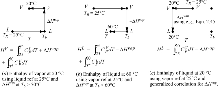
Figure 2.6. Illustrations of state pathways to calculate properties involving liquid/vapor phase changes. The examples are representative, and modified paths would apply for states above the normal boiling point, Tb. Similar pathways apply for solid/liquid or solid/vapor transformations. Note that a generalized correlation is used for ΔHvap which differs from the normal boiling point value. The method is intended to be used at subcritical conditions. Pressure corrections are not illustrated for any paths here.
Example 2.8. Acetone enthalpy using various reference states
Calculate the enthalpy values for acetone as liquid at 20°C and vapor at 90°C and the difference in enthalpy using the following reference states: (a) liquid at 20°C; (b) ideal gas at 25°C and ΔHvap at the normal boiling point; (c) ideal gas at 25°C and the generalized correlation for ΔHvap at 20°C. Ignore pressure corrections and treat vapors as ideal gases.
Solution
Heat capacity constants are available in Appendix E. For all cases, 20°C is 293.15K, 90°C is 363.15K, and the normal boiling point is Tb = 329.15K.
a. HL = 0 because the liquid is at the reference state. The vapor enthalpy is calculated analogous to Fig. 2.6, pathway (a). The three terms of pathway (a) are HV = 4639 + 30200 + 2799 = 37,638 J/mol. The difference in enthalpy is ΔH = 37,638 J/mol.
b. HL will use a path analogous to Fig. 2.6, pathway (b). The three terms of pathway (b) are HL = 2366 – 30200 – 4638 = –32472 J/mol. HV is calculated using Eqn. 2.50, HV = 5166 J/mol. The difference is ΔH = 5166 + 32472 = 37,638 J/mol, same as part (a).
c. HL will use a path analogous to Fig. 2.6, pathway (c). The generalized correlation of Eqn. 2.45 predicts a heat of vaporization at Tb of 29,280 J/mol, about 3% low. At 20°C, the heat of vaporization is predicted to be 31,420 J/mol. The two steps in Fig. 2.6 (c) are HL = –365 – 31420 = –31785 J/mol. The enthalpy of vapor is the same calculated in part (b), HV = 5166 J/mol. The enthalpy difference is ΔH = 5166 + 31785 = 36,950 J/mol, about 2% low relative to part (b).
2.12. Kinetic and Potential Energy
The development of the energy balance includes potential and kinetic energy terms for the system and for streams crossing the boundary. When temperature changes occur, the magnitude of changes of U and H are typically so much larger than changes in kinetic and potential energy that the latter terms can be dropped. The next example demonstrates how this is justified.
Example 2.9. Comparing changes in kinetic energy, potential energy, internal energy, and enthalpy
For a system of 1 kg water, what are the internal energy and enthalpy changes for raising the temperature 1°C as a liquid and as a vapor from 24°C to 25°C? What are the internal energy enthalpy changes for evaporating from the liquid to the vapor state? How much would the kinetic and potential energy need to change to match the magnitudes of these changes?
Solution
The properties of water and steam can be found from the saturated steam tables, interpolating between 20°C and 25°C. For saturated water or steam being heated from 24°C to 25°C, and for vaporization at 25°C:
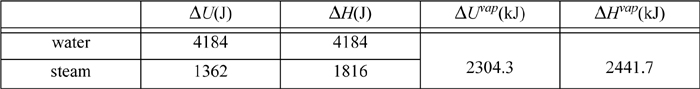
Of these values, the values for ΔU of steam are lowest and can serve as the benchmark. How much would kinetic and potential energy of a system have to change to be comparable to 1000 J?
Kinetic energy: If ΔKE = 1000 J, and if the kg is initially at rest, then the velocity change must be,
This corresponds to a velocity change of 161 kph (100 mph). A velocity change of this order of magnitude is unlikely in most applications except nozzles (discussed below). Therefore, kinetic energy changes can be neglected in most calculations when temperature changes occur.
Potential energy: If ΔPE = 1000 J, then the height change must be,
This is equivalent to about one football field in position change. Once again this is very unlikely in most process equipment, so it can usually be ignored relative to heat and work interactions. Further, when a phase change occurs, these changes are even less important relative to heat and work interactions.
![]() Velocity and height changes must be large to be significant in the energy balance when temperature changes also occur.
Velocity and height changes must be large to be significant in the energy balance when temperature changes also occur.
Example 2.9 demonstrates that kinetic and potential energy changes of a fluid are usually negligible when temperature changes by a degree or more. Moreover, kinetic and potential energy changes are closely related to one another in the design of piping networks because the temperature changes are negligible. The next example helps illustrate the point.
Example 2.10. Transformation of kinetic energy into enthalpy
Water is flowing in a straight horizontal pipe of 2.5 cm ID with a velocity of 6.0 m/s. The water flows steadily into a section where the diameter is suddenly increased. There is no device present for adding or removing energy as work. What is the change in enthalpy of the water if the downstream diameter is 5 cm? If it is 10 cm? What is the maximum enthalpy change for a sudden enlargement in the pipe? How will these changes affect the temperature of the water?
Solution
A boundary will be placed around the expansion section of the piping. The system is fixed volume, (![]() ), adiabatic without shaft work. The open steady-state system is under steady-state flow, so the left side of the energy balance is zero.
), adiabatic without shaft work. The open steady-state system is under steady-state flow, so the left side of the energy balance is zero.

Simplifying: ![]()
Liquid water is incompressible, so the volume (density) does not change from the inlet to the outlet. Letting A represent the cross-sectional area, and letting D represent the pipe diameter,![]() ,
,
D2/D1 = 2 ⇒ ΔH = –6.02 m2/s2 (1J/1kg-m2/s2) (½4–1)/2 = 17 J/kg
D2/D1 = 4 ⇒ ΔH = 18 J/kg
D2/D1 = ∞ ⇒ ΔH = 18 J/kg
To calculate the temperature rise, we can relate the enthalpy change to temperature since they are both state properties. From Eqn. 2.42, neglecting the effect of pressure,
Example 2.10 shows that the temperature rise due to velocity changes is very small. In a real system, the measured temperature rise will be slightly higher than our calculation presented here because irreversibilities are caused by the velocity gradients and swirling in the region of the sudden enlargement that we haven’t considered. These losses increase the temperature rise. In fluid mechanics, irreversible losses due to flow are characterized by a quantity known as the friction factor. The losses of a valve, fitting, contraction, or enlargement can be characterized empirically by the equivalent length of straight pipe that would result in the same losses. We will introduce these topics in Section 5.7. However, we conclude that from the standpoint of the energy balance, the temperature rise is still small and can be neglected except in the most detailed analysis such as the design of the piping network. In Example 2.10 the velocity decreases, and enthalpy increases due to greater flow work on the inlet than the outlet. Note that the above result for a liquid does not depend on whether the enlargement is rapid or gradual. A gradual taper will give the same temperature change since the energy balance relates the enthalpy change to the initial and final velocities, but not on the manner in which the change occurs.
Applications where kinetic and potential energy changes are important include solids such as projectiles, where the temperature changes of the solids are negligible and the purpose of the work is to cause accelerate or elevate the system. One example of this application is a steam catapult used to assist in take-off from aircraft carriers. A steam-filled piston + cylinder device is expanded, and the piston drags the plane to a velocity sufficient for the jet engines to lift the plane. While the kinetic and potential energy changes for the steam are negligible, the work done by the steam causes important kinetic energy changes in the piston and plane because of their large masses.
2.13. Energy Balances for Process Equipment
Several types of equipment are ubiquitous throughout industry, and facile abilities with the energy balance for these processes will permit more rapid analysis of composite systems where these units are combined. In this brief section we introduce valves and throttles used to regulate flow, nozzles, heat exchangers, adiabatic turbines and expanders, adiabatic compressors, and pumps.
Valves and Throttles
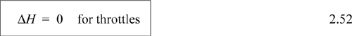
A throttling device is used to reduce the pressure of a flowing fluid without extracting any shaft work and with negligible fluid acceleration. Throttling is also known as Joule-Thomson expansion in honor of the scientists who originally studied the thermodynamics. An example of a throttle is the kitchen faucet. Industrial valves are modeled as throttles. Writing the balance for a boundary around the throttle valve, it is conventional to neglect any accumulation within the device since it is small relative to flow rates through the device, so the left-hand side is zero. At steady-state flow,
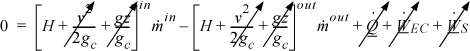
Changes in kinetic and potential energy are small relative to changes in enthalpy as we just discussed. When in doubt, the impact of changes in velocity can be evaluated as described in Example 2.9. The amount of heat transfer is negligible in a throttle. The boundaries are not expanding, and there is also no mechanical device for transfer of work, so the work terms vanish. Therefore, a throttle is isenthalpic:
Nozzles
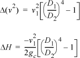
Nozzles are specially designed devices utilized to convert pressure drop into kinetic energy. Common engineering applications involve gas flows. An example of a nozzle is a booster rocket. Nozzles are also used on the inlets of impulse turbines to convert the enthalpy of the incoming stream to a high velocity before it encounters the turbine blades.13 Δu is significant for nozzles. A nozzle is designed with a specially tapered neck on the inlet and sometimes the outlet as shown schematically in Fig. 2.7. Nozzles are optimally designed at particular velocities/pressures of operation to minimize viscous dissipation.
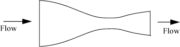
Figure 2.7. Illustration of a converging-diverging nozzle showing the manner in which inlets and outlets are tapered.
The energy balance is written for a boundary around the nozzle. Any accumulation of energy in the nozzle is neglected since it is small relative to flow through the device and zero at steady state. Velocity changes are significant by virtue of the design of the nozzle. However, potential energy changes are negligible. Heat transfer and work terms are dropped as justified in the discussion of throttles. Reducing the energy balance for a nozzle shows the following:
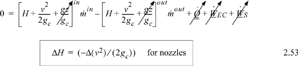
Properly designed nozzles cause an increase in the velocity of the vapor and a decrease in the enthalpy. A nozzle can be designed to operate nearly reversibly. Example 4.12 on page 162 describes a typical nozzle calculation.
Throttles are much more common in the problems we will address in this text. The meaning of “nozzle” in thermodynamics is much different from the common devices we term “nozzles” in everyday life. Most of the everyday devices we call nozzles are actually throttles.
Assessing when simplifications are justified requires testing the implications of eliminating assumptions. For example, to test whether a particular valve is acting more like a throttle or a nozzle, infer the velocities before and after the nozzle and compare to the enthalpy change. If the kinetic energy change is negligible relative to the enthalpy change then call it a throttle. Take note of the magnitude of the terms in the calculation so that you can understand how to anticipate a similar conclusion. For example, the volume change of a liquid due to a pressure drop is much smaller than that of a gas. With less expansion, the liquids accelerate less, making the throttle approximation more reasonable. This kind of systematic analysis and reasoning is more important than memorizing, say, that throttles are for liquids.
Heat Exchangers
Heat exchangers are available in a number of flow configurations. For example, in an industrial heat exchanger, a hot stream flows over pipes that carry a cold stream (or vice versa), and the objective of operation is to cool one of the streams and heat the other. A generic tube-in-shell heat exchanger can be illustrated by a line diagram as shown in Fig. 2.8. Tube-in-shell heat exchangers consist of a shell (or outer sleeve) through which several pipes pass. (The figure just has one pipe for simplicity.) One of the process streams passes through the shell, and the other passes through the tubes. Stream A in our example passes through the shell, and Stream B passes through the tubes. The streams are physically separated from one another by the tube walls and do not mix. Let’s suppose that Stream A is the hot stream and Stream B is the cold stream. In the figure, both streams flow from left to right. This type of flow pattern is called concurrent. The temperatures of the two streams will approach one another as they flow to the right. With this type of flow pattern, we must be careful that the hot stream temperature that we calculate is always higher than the cold stream temperature at every point in the heat exchanger.14 If we reverse the flow direction of Stream A, a countercurrent flow pattern results. With a countercurrent flow pattern, the outlet temperature of the cold stream can be higher than the outlet temperature of the hot stream (but still must be lower than the inlet temperature of the hot stream). The hot stream temperature must always be above the cold stream temperature at all points along the tubes in this flow pattern also.

Figure 2.8. Illustration of a generic heat exchanger with a concurrent flow pattern. The tube side usually consists of a set of parallel tubes which are illustrated as a single tube for convenience.
So far, our discussion has assumed that there are no phase transitions occurring in the heat exchanger. If Stream A is a hot stream, and Stream B is converted from liquid at the inlet to vapor at the outlet, we call the heat exchanger a boiler to bring attention to the phase transition occurring inside. The primary difference in the operation of a boiler to that of a generic heat exchanger is that the cold stream temperature change might be small or even zero. This is because the phase change will occur isothermally at the saturation temperature of the fluid corresponding to the boiler pressure, absorbing large amounts of heat. In a similar fashion, we could have Stream A be cooling water and Stream B be an incoming vapor which is condensed. We would call this heat exchanger a condenser, to clearly bring attention to the phase change occurring inside. In this case, the temperature change of the hot stream might be small. Another type of heat exchanger that we will use in Chapter 5 is the superheater. A superheater takes a vapor that is saturated and superheats it.
There are two more important points to keep in your mind as you perform thermodynamic calculations. For the purposes of this text we will neglect pressure drops in the heat exchangers; the outlet pressure will match the inlet pressure of Stream A, and a similar statement applies for Stream B. Note that this does not imply that streams A and B are at the same pressure. Also, we neglect heat transfer to or from the surroundings unless specified. Therefore, all heat transfer occurs inside the heat exchanger, not at the boundaries of the heat exchanger and the surroundings.
There are other configurations of heat exchangers such as kettle-type reboilers and plate-and-frame configurations; however, for thermodynamic purposes, only the flow pattern is important, not the details of material construction that lead to the flow pattern. Thus, the tube-in-shell concepts will be adequate for our needs.
The energy balance that we write depends on how we choose our system. Since the streams are physically separated from one another, we may write a balance for each of the streams independently, or we may place the system boundary around the entire heat exchanger and write a balance for both streams. Let us take the system to be Stream B and let us suppose that Stream B is boiled. In this case, there is just one inlet and outlet. There is no shaft work or expansion/contraction work. Even though the process fluid is expanding as it evaporates, the system boundaries are not expanding; expansion effects will be automatically included in the energy balance by the enthalpy terms which have the flow work embedded in them. If the system is operating at steady state, the left-hand side of the energy balance is zero,
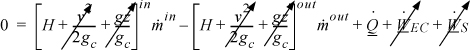
which simplifies to
where ![]() is the rate of heat transfer from the hot stream. On a molar (or mass) basis,
is the rate of heat transfer from the hot stream. On a molar (or mass) basis,
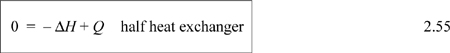
If we take the system boundaries to be around the entire heat exchanger, then there are multiple streams, and all heat transfer occurs inside, resulting in
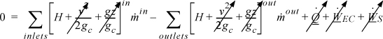
which simplifies to
Since Eqns. 2.55 and 2.57 look quite different for the same process, it is important that you understand the placement of boundaries and their implications on the balance expression.
Adiabatic Turbines or Adiabatic Expanders
A turbine or expander is basically a sophisticated windmill as shown in Fig. 2.9. The term “turbine” implies operation by steam and the term “expander” implies operation by a different process fluid, perhaps a hydrocarbon, although the term “turbine” is used sometimes for both. The objective of operation is to convert the kinetic energy from a gas stream to rotary motion of a shaft to produce work (shaft work). The enthalpy of the high-pressure inlet gas is converted to kinetic energy by special stators (stationary blades) or nozzles inside the turbine shell. The high-velocity gas drives the rotor. Turbines are designed to be adiabatic, although heat losses can occur. When heat losses are present, they decrease the output that would have otherwise been possible for the turbine. Therefore, when calculations are performed, we assume that turbines or expanders operate adiabatically, unless otherwise noted.
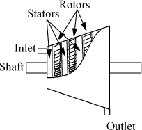
Figure 2.9. Illustration of a turbine. The rotor (shaft) turns due to the flow of gas. The blades connected to the shell are stationary (stators), and are sometimes curved shapes to perform as nozzles. The stator blades are not shown to make the rotors more clear.
The energy balance for the turbine only involves the kinetic energy change for the entering and exiting fluid, not for the changes occurring inside the turbine. Since the nozzles which cause large kinetic energy changes are inside the turbine unit, these changes are irrelevant to the balance around the unit. Recall from the development of our energy balance that we are only interested in the values of enthalpy, kinetic, and potential energy for streams as they cross the boundaries of our system. The energy balance for a steady-state turbine involving one inlet and one outlet is:
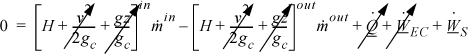
which becomes
and on a mass or molar basis becomes
When we calculate values for the ΔH and work, they will be negative values.
Adiabatic Compressors
Adiabatic compressors can be constructed in a manner qualitatively similar to adiabatic turbines with stationary vanes (stators). This type of compressor is called an axial compressor. The main differences between turbines and axial compressors are: 1) the details of the construction of the vanes and rotors, which we won’t be concerned with; 2) the direction of flow of the fluid; and 3) the fact that we must put work into the compressor rather than obtaining work from it. Thus, the energy balance is the same as the turbine (Eqns. 2.58 and 2.59). When we calculate values for the ΔH and work, they will be positive values, where they were negative values for a turbine. Compressors may also be constructed as reciprocating (piston/cylinder) devices. This modification has no impact on our energy balance, so it remains the same. Analogous to turbines, it is conventional to assume that compressors are adiabatic unless otherwise noted.
Pumps
Pumps are used to move liquids by creating the pressure necessary to overcome the resistance to flow. They are in principle just like compressors, except the liquid will not change density the way a gas does when it is compressed. Again, the energy balance will be the same as a turbine or compressor (Eqns. 2.58 and 2.59). The primary difference we will find in application of the energy balance is that tabulated enthalpies are difficult to find for compressed liquids. Therefore, if we want to calculate the work needed for a pump, we can find it from the energy balance after we have calculated or determined the enthalpy change.
Calculation of Shaft Work
Adiabatic steady-state turbines, compressors, and pumps all share a common energy balance, showing that the shaft work is related to the enthalpy change as shown on page 54. Often, it is helpful to calculate the shaft work directly and use the value of the shaft work to find the enthalpy change.
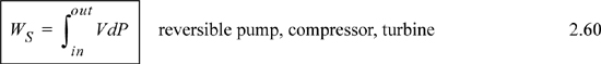
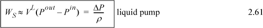
When the work is to calculated, the adiabatic shaft work may, in principle, be analyzed using ΔH or Eqn 2.60. For gases, it is usually easier to use other constraints to find the enthalpy change and then calculate the work by equality, though in principle the integral can be evaluated. For the special case of liquids, Eqn 2.60 can be replaced by Eqn. 2.61.
2.14. Strategies for Solving Process Thermodynamics Problems
Before we start several more complicated example problems, it will be helpful to outline the strategies which will be applied. We provide these in a step form to make them easier to use. Many of these steps will seem obvious, but if you become stuck when working through a problem, it is usually because one of these steps was omitted or applied inconsistently with system boundaries.
1. Choose system boundaries; decide whether this boundary location will make the system open or closed.
2. Identify all given state properties of fluids in system and crossing boundaries. Identify which are invariant with time. Identify your system as steady or unsteady state. (For unsteady-state pumps, turbines, or compressors, the accumulation of energy within the device is usually neglected.) For open, steady-state systems, write the mass balance and solve if possible.
3. Identify how many state variables are unknown for the system. Recall that only two state variables are required to specify the state of a pure, single-phase fluid. The number of unknowns will equal the number of independent equations necessary for a solution. (Remember in a system of known total volume V, that if n is known, the state variable V is known.)
4. Write the mass balance and the energy balance. These are the first equations to be used in the solution. Specify reference states for all fluids if necessary. Simplify energy balance to eliminate terms which are zero for the system specified in step 1.15 Combine the mass balance and the energy balance for open systems.
For unsteady-state problems:
a. Identify whether the individual terms in the energy balance may be integrated directly without combining with other energy balance terms. Often the answer is obtained most easily this way. This is almost always possible for closed-system problems.
b. If term-by-term integration of the energy balance is not possible, rearrange the equation to simplify as much as possible before integration.
5. Look for any other information in the problem statement that will provide additional equations if unknowns remain. Look for key words such as adiabatic, isolated, throttling, nozzle, reversible, and irreversible. Using any applicable constraints of throttling devices, nozzles, and so on, relate stream properties for various streams to one another and to the system state properties. Constraints on flow rates, heat flow, and so on. provide additional equations. With practice, many of these constraints may be recognized immediately before writing the energy balance in steps 3 and 4.
6. Introduce the thermodynamic properties of the fluid (the equation of state). This provides all equations relating P, V, T, U, H, CP, and CV. The information will consist of either 1) the ideal gas approximation; 2) a thermodynamic chart or table; or 3) a volumetric equation of state (which will be introduced in Chapter 7). Using more than one of these sources of information in the same problem may introduce inconsistencies in the properties used in the solution, depending on the accuracy of the methods used.
Combine the thermodynamic information with the energy balance. Work to minimize the number of state variables which remain unknown. Many problems are solved at this point.
7. Do not hesitate to move your system boundary and try again if you are stuck. Do not forget to try an overall balance (frequently, two open systems can be combined to give an overall closed system, and strategy 4a can be applied). Make reasonable assumptions.
8. After an answer is obtained, verify assumptions that were made to obtain the solution.
2.15. Closed and Steady-State Open Systems
Several types of systems are quite common in chemical engineering practice. You need to be familiar with the results of their analysis and benefit if you memorize these results for rapid recall. You must simultaneously recall the assumptions underlying each simple model, however, to avoid incorrect applications.
Example 2.11. Adiabatic, reversible expansion of an ideal gas
Suppose an ideal gas in a piston + cylinder is adiabatically and reversibly expanded to twice its original volume. What will be the final temperature?
Solution
First consider the energy balance. The system will be the gas in the cylinder. The system will be closed. Since a basis is not specified, we can choose 1 mole. Since there is no mass flow, heat transfer, or shaft work, the energy balance becomes:

In this case, as we work down to step 4 in the strategy, we see that we cannot integrate the sides independently since P depends on T. Therefore, we need to combine terms before integrating.
The technique that we have performed is called separation of variables. All of the temperature dependence is on the left-hand side of the equation and all of the volume dependence is on the right-hand side. Now, if we assume a constant heat capacity for simplicity, we can see that this integrates to
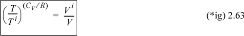
![]() These boxed equations relate state variables for adiabatic reversible changes of an ideal gas in a closed system.
These boxed equations relate state variables for adiabatic reversible changes of an ideal gas in a closed system.
Although not required, several rearrangements of this equation are useful for other problems. Note that we may insert the ideal gas law to convert to a formula relating T and P. Using V = RT/P,
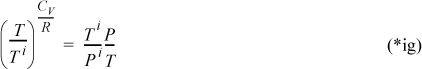
Rearranging,

which becomes
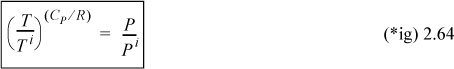
We may also insert the ideal gas law into Eqn. 2.63 to convert to a formula relating P and V. Using T = PV/R,
which may be written
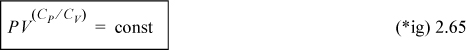
The analysis of a piston+cylinder implied the assumption of a closed system. This might be a reasonable approximation for a single stroke of a combustion engine, but most chemical engineering applications involve continuous operation. Nevertheless, we can apply the lessons learned from the analysis of the closed system when extending to steady-state systems, as exemplified below.
Example 2.12. Continuous adiabatic, reversible compression of an ideal gas
Suppose 1 kmol/h of air at 5 bars and 298 K is adiabatically and reversibly compressed in a continuous process to 25 bars. What will be the outlet temperature and power requirement for the compressor in hp?
Note that air is composed primarily of oxygen and nitrogen and these both satisfy the stipulations for diatomic gases with their reduced temperatures high and their reduced pressures low. In other words, the ideal gas approximation with CP/R = 7/2 is clearly applicable. Next consider the energy balance. The system is the compressor. The system is open. Since it is a steady-state process with no heat transfer, the simplification of the energy balance has been discussed on page 73 and shown on page 72, and the energy balance becomes:

We can adapt Eqn. 2.31 for an ideal gas as follows:
dWS = dH = VdP
In this case, as we work down to step 4 in the strategy, we see that we cannot integrate the sides independently since P depends on T. Therefore, we need to combine terms before integrating.
Once again, we have performed separation of variables. The rest of the derivation is entirely analogous to Example 2.11, and, in fact, the resultant formula is identical.
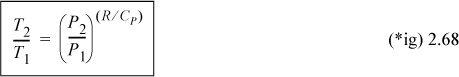
![]() Steady-state adiabatic, reversible processing of an ideal gas results in the same relations as Example 2.11.
Steady-state adiabatic, reversible processing of an ideal gas results in the same relations as Example 2.11.
Note that this formula comes up quite often as an approximation for both open and closed systems. Making the appropriate substitutions,
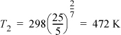
Adapting the adiabatic energy balance and assuming CPig = constant,
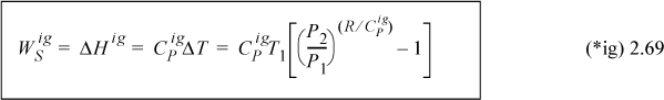
Substituting, WS = 3.5·8.314·(472–298) = 5063 J/mole
At the given flow rate, and reiterating that this problem statement specifies a reversible process:
WSrev = 5063 J/mole·[1000mole/hr]·[1hr/3600sec]·[1hp/(745.7J/s)] = 1.9hp
We have systematically extended our analysis from a single step of a closed system, to a continuous system with no heat loss. Let’s consider isothermal operation.
Example 2.13. Continuous, isothermal, reversible compression of an ideal gas
Repeat the compression from the previous example, but consider steady-state isothermal compression. What will be the heat removal rate and power requirement for the compressor in hp?
Solution
Let’s return to the perspective of the section ‘Understanding Enthalpy and Shaft Work’ on page 54 and analyze the EC work and flow work for an ideal gas packet of unit mass. The WEC is,
For an isothermal, ideal gas, V2/V1 = P1/P2. Noting the reciprocal and negative logarithm,
This is the work to isothermally squeeze an ideal gas packet of unit mass to a given pressure. The flow work performed on an ideal gas packet of unit mass is,
Therefore, the total requirement for isothermally compressing an ideal gas packet of unit mass is,
At the given flow rate, and reiterating that this problem statement specifies a reversible process,
WSrev = 3987 J/mole·[1000mole/hr]·[1hr/3600sec]·[1hp/745.7J/s] = 1.5 hp
Compared to adiabatic compression, the isothermal compressor requires less work. This happens because cooling withdraws energy from the system. It is difficult to achieve perfectly adiabatic or isothermal operation in practice, but adiabatic operation is usually a better approximation because compression is so rapid that there is insufficient time for heat transfer. Usually fluids are cooled after compression as we discuss in later chapters.
Here is a brain teaser. Suppose the process fluid had been steam instead of an ideal gas. How would you have solved the problem then? Note, for steam V ≠ RT/P and ![]() . We illustrate the answer in Example 4.16 on page 173.
. We illustrate the answer in Example 4.16 on page 173.
Example 2.14. Heat loss from a turbine
High-pressure steam at a rate of 1100 kg/h initially at 3.5 MPa and 350°C is expanded in a turbine to obtain work. Two exit streams leave the turbine. Exiting stream (2) is at 1.5 MPa and 225°C and flows at 110 kg/h. Exiting stream (3) is at 0.79 MPa and is known to be a mixture of saturated vapor and liquid. A fraction of stream (3) is bled through a throttle valve to 0.10 MPa and is found to be 120°C. If the measured output of the turbine is 100 kW, estimate the heat loss of the turbine. Also, determine the quality of the steam in stream (3).
Solution
First draw a schematic. Designate boundaries. Both System A and System B are open steady-state systems.

The mass balance gives ![]() . Next, determine which streams are completely specified: Streams (1), (2), and (4) are fully specified. Since Stream (3) is saturated, the temperature and pressure and specific enthalpies of the saturated vapor and liquid can be found, but the quality needs to be calculated to determine the overall molar enthalpy of the stream. From the steam tables we find H1 directly. For H2 we use linear interpolation. The value H(1.5 MPa, 225°C) is not available directly, so we need to first interpolate at 1.4 MPa between 200°C and 250°C to find H(1.4 MPa, 225°C) and then interpolate between this value and the value at 1.6 MPa:
. Next, determine which streams are completely specified: Streams (1), (2), and (4) are fully specified. Since Stream (3) is saturated, the temperature and pressure and specific enthalpies of the saturated vapor and liquid can be found, but the quality needs to be calculated to determine the overall molar enthalpy of the stream. From the steam tables we find H1 directly. For H2 we use linear interpolation. The value H(1.5 MPa, 225°C) is not available directly, so we need to first interpolate at 1.4 MPa between 200°C and 250°C to find H(1.4 MPa, 225°C) and then interpolate between this value and the value at 1.6 MPa:
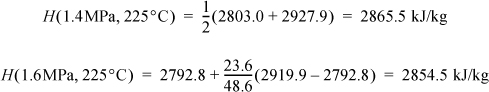
Then to find H2: H2 = 0.5·(2865.5 + 2854.5) = 2860.0 kJ/kg. For H4 we can interpolate in the superheated steam tables:
Recognize System B as a throttle valve; therefore, H3 = H4 = 2716.1 kJ/kg. We make a table to summarize the results so that we can easily find values:
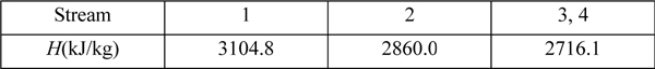
The energy balance for System A gives, using ![]() given in the problem statement,
given in the problem statement,
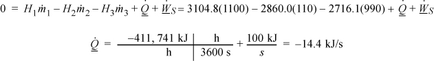
To find the quality of stream (3), ![]()
At 0.79 MPa from the sat’d P table, HL = 718.5 kJ/kg and ΔHV = 2049 kJ/kg.
The energy balance for a non-adiabatic turbine is identical to the balance for an isothermal compressor, but the conclusions are entirely different. In the compressor, we want to minimize work, so the heat loss works to our advantage. For the turbine, we want to maximize work, so any loss of energy should be avoided.
The examples in this section comprise several important common scenarios, but they also illustrate a procedure for analyzing systems with systematically increasing sophistication. In the context of certain simplifying assumptions, like the ideal gas model, we can derive final working equations applicable to process calculations. When those assumptions are invalid, however, we can still apply the energy balance, but we are more careful in the generality of the results we obtain. Processes involving steam, for example, require something more than the ideal gas model, and additional tools are required to develop a general analysis.
2.16. Unsteady-State Open Systems
In principle, most real systems are unsteady and open. A few systems couple the unsteady-state operation with flow across boundaries in a way that requires simultaneous analysis. We illustrate how to treat those systems with examples of leaking and filling tanks.
Example 2.15. Adiabatic expansion of an ideal gas from a leaky tank
An ideal gas is leaking from an insulated tank. Relate the change in temperature to the change in pressure for gas leaking from a tank. Derive an equation for ΔU for the tank.
Solution
Let us choose our system as the gas in the tank at any time. This will be an open, unsteady-state system. There is no inlet stream and one outlet stream. The mass balance gives dn = – dnout.
We can neglect kinetic and potential energy changes. Although the gas is expanding, the system size remains unchanged, and there is no expansion/contraction work. The energy balance becomes (on a molar basis):
Since the enthalpy of the exit stream matches the enthalpy of the tank, Hout = H. d(nU) = –Houtdnout = Hdn. Now H depends on temperature, which is changing, so we are not able to apply hint 4(a) from the problem-solving strategy. It will be necessary to combine terms before integrating. By the product rule of differentiation, the left-hand side expands to d(nU) = ndU + Udn. Collecting terms in the energy balance,
ndU = (H – U)dn
Performing some substitutions, the energy balance can be written in terms of T and n,
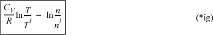
The volume of the tank is constant, (V = constant); therefore,
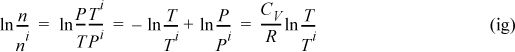
substituting,
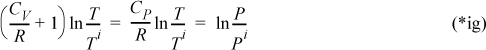
Recognizing the relation between CV and CP, defining γ≡ Cp/Cv (=1.4 for an ideal diatomic gas), note R/Cp = (Cp – CV)/CP = 1 – (1/γ) = (γ – 1)/γ:

Through the ideal gas law (PV = RT), we can obtain other arrangements of the same formula.
The numerical value for the change in internal energy of the system depends on the reference state because the reference state temperature will appear in the result:
![]() For fluid exiting from an adiabatic tank, the results are the same as a closed system as in Example 2.11.
For fluid exiting from an adiabatic tank, the results are the same as a closed system as in Example 2.11.
At first glance, one might expect to use the same equation for a filling tank, but simply change the pressure ratio. Careful analysis shows that the energy balance is similar, but the final result is quite different.
Example 2.16. Adiabatically filling a tank with an ideal gas
Helium at 300 K and 3000 bar is fed into an evacuated cylinder until the pressure in the tank is equal to 3000 bar. Calculate the final temperature of the helium in the cylinder (CP/R = 5/2).
Solution
The system will be the gas inside the tank at any time. The system will be an open, unsteady-state system. The mass balance is dn = dnin. The energy balance becomes:
We recognize that Hin will be constant throughout the tank filling. Therefore, by hint 4a from the problem-solving strategy, we can integrate terms individually. We need to be careful to keep the superscript since the incoming enthalpy is at a different state than the system. The right-hand side of the energy balance can be integrated to give
The left-hand side of the energy balance becomes
Δ(Un) = Ufnf – Uini = Ufnf
Combining the result with the definition of enthalpy,
And with our definition of heat capacity, we can find temperatures:
Note that the final temperature is independent of pressure for the case considered here.
You should not get the impression that unsteady, open systems are limited to ideal gases. Energy balances are independent of the type of operating fluid.
Example 2.17. Adiabatic expansion of steam from a leaky tank
An insulated tank contains 500 kg of steam and water at 215°C. Half of the tank volume is occupied by vapor and half by liquid; 25 kg of dry vapor is vented slowly enough that temperature remains uniform throughout the tank. What is the final temperature and pressure?
Solution
There are some similarities with the solution to Example 2.15 on page 81; however, we can no longer apply the ideal gas law. The energy balance reduces in a similar way, but we note that the exiting stream consists of only vapor; therefore, it is not the overall average enthalpy of the tank:
d(mU) = –Houtdmout = HV dm
The sides of the equation can be integrated independently if the vapor enthalpy is constant. Looking at the steam table, the enthalpy changes only about 10 kJ/kg out of 2800 kJ/kg (0.3%) along the saturation curve down to 195°C. Let us assume it is constant at 2795 kJ/kg making the integral of the right-hand side simply HVΔm. Note that this procedure is equivalent to a numerical integration by trapezoidal rule as given in Appendix B on page 822. Many students forget that analytical solutions are merely desirable, not absolutely necessary. The energy balance then can be integrated using hint 4a on page 74.
ΔU = mfUf – miUi = 2795(mf – mi) = 2795(–25) = –69,875 kJ
The quantity mf = 475, and miUi will be easy to find, which will permit calculation of Uf. For each m3 of the original saturated mixture at 215°C,
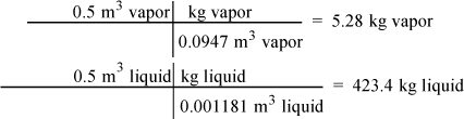
So the tank volume, quality, and internal energy are:
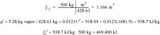
Then, from the energy balance and mass balance,
Uf = (–69,875 + 469,400) kJ / 475 kg = 841.0 kJ/kg
Vf = 1.166 m3 / 475 kg = 0.00245 m3/kg
We need to find Pf and Tf which correspond to these state variables. The answer will be along the saturation curve because the overall specific volume is intermediate between saturated vapor and liquid values at lower pressures. We will guess Pf (and the corresponding saturation Tf), find q from Vf, then calculate ![]() and compare to Uf = 841.0 kJ/kg. If
and compare to Uf = 841.0 kJ/kg. If ![]() is too high, the Pf (and Tf) guess will be lowered.
is too high, the Pf (and Tf) guess will be lowered.
Since V = VL + q(VV–VL),
To guide our first guess, we need UL < Uf = 841.0 kJ/kg. Our first guess is Tf = 195°C. Values for the properties from the steam tables are shown in the table below. This initial guess gives Ufcalc = 845 kJ/kg; no further iteration is necessary. The HV at this state is 2789; therefore, our assumption of Hout ≈ constant is valid.
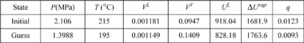
Pf = 1.4 MPa, Tf = 195°C, ΔP = 0.7 MPa, ΔT = 20°C
2.17. Details of Terms in the Energy Balance
Generally, the strategies discussed in Section 2.14 are sufficient to simplify the energy balance. Occasionally, in applying the energy balance to a new type of system, simplification of the balances may require more detailed analysis of the background leading to the terms and/or details of interactions at boundaries. This section provides an overall summary of the details for the principles covered earlier in this chapter, and it is usually not necessary unless you are having difficulty simplifying the energy balance and need details regarding the meaning of each term.
The universe frequently consists of three subsystems, as illustrated in Fig. 2.10. The container (System 2) is frequently combined with System 1 (designated here as System (1 + 2)) or System 3 (designated here as System (2 + 3)). For every balance, all variables are of the system for which the balance is written,


Figure 2.10. Schematic of a general system.
where superscripts “in” and “out” denote properties of the streams which cross the boundaries, which may or may not be equal to properties of the system.
1. Non-zero heat interactions of Systems 1 and 3 are not equal unless the heat capacity or mass of System 2 is negligible.
2. Hout, Hin account for internal energy changes and work done on the system due to flow across boundaries.
3. ![]() represents work done on the system due to expansion or contraction of system size. Fboundary is the absolute value of the system force at the boundary. (By Newton’s third principle, the forces are equal but act in opposite directions at any boundary.) Note that system 1 and system 3 forces are not required to be equal. Unequal forces create movement (acceleration) of any movable barrier (e.g., piston head).
represents work done on the system due to expansion or contraction of system size. Fboundary is the absolute value of the system force at the boundary. (By Newton’s third principle, the forces are equal but act in opposite directions at any boundary.) Note that system 1 and system 3 forces are not required to be equal. Unequal forces create movement (acceleration) of any movable barrier (e.g., piston head).
4. ![]() represents the work done on the system resulting from mechanical forces at the surface of the system except work due to expansion/contraction or mass flow across boundaries. Turbines and compressors are part of system 2; thus they are involved with work interactions with the fluid in system 1. Note that piston movement is calculated as
represents the work done on the system resulting from mechanical forces at the surface of the system except work due to expansion/contraction or mass flow across boundaries. Turbines and compressors are part of system 2; thus they are involved with work interactions with the fluid in system 1. Note that piston movement is calculated as ![]() for systems 1, 3, (1+2), or (2+3), but the movement is calculated as
for systems 1, 3, (1+2), or (2+3), but the movement is calculated as ![]() for system 2 alone. When a balance for system 2 is considered, the movement of the piston is technically shaft work, even though no shaft is involved. (The piston is a closed system, and it does not expand or contract when it moves.) As another example of the general definition of shaft work as it relates to forces at the surface of a system, consider the closed system of Fig. 2.3 on page 48 being raised 150 m or accelerated to 75 m/s. There is a work interaction at the surface of the system required for these energy changes even though there is not a “rotating” shaft.
for system 2 alone. When a balance for system 2 is considered, the movement of the piston is technically shaft work, even though no shaft is involved. (The piston is a closed system, and it does not expand or contract when it moves.) As another example of the general definition of shaft work as it relates to forces at the surface of a system, consider the closed system of Fig. 2.3 on page 48 being raised 150 m or accelerated to 75 m/s. There is a work interaction at the surface of the system required for these energy changes even though there is not a “rotating” shaft.
5. Non-zero ![]() or
or ![]() interactions of systems 1 and 3 are not equal unless changes in kinetic and potential energy of the moving portion of system 2 (e.g., piston head for
interactions of systems 1 and 3 are not equal unless changes in kinetic and potential energy of the moving portion of system 2 (e.g., piston head for ![]() or turbine for
or turbine for ![]() ) are negligible and the movement is reversible.
) are negligible and the movement is reversible.
6. Frictional forces, if present, must be attributed to one of the systems shown above. Irreversibility due to any cause does not require additional energy balance terms because energy is always conserved, even when processes are irreversible.
7. Electrical and magnetic fields have not been included.
8. On the left-hand side of the equation, kinetic and potential energy changes are calculated based on movement of the center of mass. In a composite system such as (1+2), they may be calculated for each subsystem and summed.
2.18. Summary
We are trying to be very careful throughout this chapter to anticipate every possibility that might arise. As a result, the verbiage gets very dense. Think of the complete energy balance as a checklist, reminding you to consider whether each term may contribute significantly to a given problem, and learning to translate key terms like “frictionless,” “reversible,” “continuous,” and “steady state” into meaningful reductions of the balance.
Important Equations
If we relax the formality, we can summarize most of this chapter casually as follows:
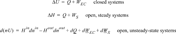
Naturally, it is best to appreciate how these equations result from simplifications. Remember to check the general energy balance for terms that may be significant in exceptional situations.
A summary of expansion/contraction work relations for ideal gases is also presented here, however it is recommended that you become proficient in the manipulations leading to these formulas. Section 2.4 summarizes factors that may make a process irreversible. The following formulas represent reversible work done when the system pressure is inserted for the isothermal process. The isobaric formula is the only one that can be used to directly calculate work done on the surroundings in an irreversible process, and in that case the surrounding pressure is used instead of the system pressure.

This last equation (for T2/T1) recurs frequently as we examine processes from various perspectives and simplify them to ideal gases for preliminary consideration. You should commit it to memory soon and learn to recognize when it is applicable.
Test Yourself
1. Write the energy balance without looking at the book. To help remember the terms, think about the properties the terms represent rather than memorizing the symbols.
2. In the presentation of the text, which side of the balance represents the system and which terms represent interactions at the boundaries?
3. Explain the terms “closed-system,” “open-system,” and “steady state” to a friend of the family member who is not an engineer.
4. Explain how a reference state helps to solve problems. Select a reference state for water that is different from the steam table reference state. Create a path starting from saturated liquid below the normal boiling point, through the normal boiling point, and cooling down to saturated vapor at the initial temperature. Use heat capacities and the latent heat at the normal boiling point to estimate the heat of vaporization and compare it with the steam table value.
5. Write a MATLAB, Excel, or calculator routine that will enable you to calculate heat capacity integrals easily.
6. Think of as many types of paths as you can from memory (isothermal, adiabatic, etc.) and try to derive the heat and work flow for a piston/cylinder system along each path.
2.19. Practice Problems
A. General Reductions of the Energy Balance
The energy balance can be developed for just about any process. Since our goal is to learn how to develop model equations as well as to simply apply them, it is valuable practice to obtain the appropriate energy balance for a broad range of odd applications. If you can deduce these energy balances, you should be well prepared for the more common energy balances encountered in typical chemical engineering processes.
P2.1. A pot of water is boiling in a pressure cooker when suddenly the pressure relief valve becomes stuck, preventing any steam from escaping. System: the pot and its contents after the valve is stuck. (ANS. ![]() )
)
P2.2. The same pot of boiling water as above. System: the pot and its contents before the valve is stuck. (ANS. ![]() )
)
P2.3. An gas home furnace has been heating the house steadily for hours. System: the furnace. (ANS. ![]() ) (gas furnace)
) (gas furnace)
P2.4. An gas home furnace has been heating the house steadily for hours. System: the house and all contents. (ANS. ![]() ) (gas furnace)
) (gas furnace)
P2.5. A child is walking to school when he is hit by a snowball. He stops in his tracks. System: the child. (ANS. Δ[mU + mV2 / 2gc] = msnow[H + v2 / (2gc)]snow)
P2.6. A sealed glass bulb contains a small paddle-wheel (Crookes radiometer). The paddles are painted white on one side and black on the other. When placed in the sun, the paddle wheel begins to turn steadily. System: the bulb and its contents. (ANS. ΔU = 0)
P2.7. A sunbather lays on a blanket. At 11:30 A.M., the sunbather begins to sweat. System: the sunbather at noon. (ANS. ![]() )
)
P2.8. An inflated balloon slips from your fingers and flies across the room. System: balloon and its contents. (ANS. d[mU + mv2balloon/2gc]/dt = [H + v2 / (2gc)]outdm/dt + WEC)
B. Numerical Problems
P2.9. Consider a block of concrete weighing 1 kg.
a. How far must it fall to change its potential energy by 1 kJ? (ANS. 100 m)
b. What would be the value of its velocity at that stage? (ANS. 44.7 m/s)
P2.10. A block of copper weighing 0.2 kg with an initial temperature of 400 K is dropped into 4 kg of water initially at 300 K contained in a perfectly insulated tank. The tank is also made of copper and weighs 0.5 kg. Solve for the change in internal energy of both the water and the block given CV = 4.184 J/g-K for water and 0.380 J/g-K for copper. (ANS. 7480 J, –7570 J)
P2.11. In the preceding problem, suppose that the copper block is dropped into the water from a height of 50 m. Assuming no loss of water from the tank, what is the change in internal energy of the block? (ANS. –7570 J)
P2.12. In the following take CV = 5 and CP = 7 cal/mol-K for nitrogen gas:
a. Five moles of nitrogen at 100°C is contained in a rigid vessel. How much heat must be added to the system to raise its temperature to 300°C if the vessel has a negligible heat capacity? (ANS. 5000 cal) If the vessel weighs 80 g and has a heat capacity of 0.125 cal/g-K, how much heat is required? (ANS. 7000 cal)
b. Five moles of nitrogen at 300°C is contained in a piston/cylinder arrangement. How much heat must be extracted from this system, which is kept at constant pressure, to cool it to 100°C if the heat capacity of the piston and cylinder is neglected? (ANS. 7000 cal)
P2.13. A rigid cylinder of gaseous hydrogen is heated from 300 K and 1 bar to 400 K. How much heat is added to the gas? (ANS. 2080 J/mole)
P2.14. Saturated steam at 660°F is adiabatically throttled through a valve to atmospheric pressure in a steady-state flow process. Estimate the outlet quality of the steam. (ANS. q = 0.96)
P2.15. Refer to Example 2.10 about transformation of kinetic energy to enthalpy. Instead of water, suppose N2 at 1 bar and 298 K was flowing in the pipe. How would that change the answers? In particular, how would the temperature rise change? (ANS. max ~0.001K)
P2.16. Steam at 150 bars and 600°C passes through process equipment and emerges at 100 bars and 700°C. There is no flow of work into or out of the equipment, but heat is transferred.
a. Using the steam tables, compute the flow of heat into the process equipment per kg of steam. (ANS. 288 kJ/kg)
b. Compute the value of enthalpy at the inlet conditions, Hin, relative to an ideal gas at the same temperature, Hig. Consider steam at 1 bar and 600°C as an ideal gas. Express your answer as (Hin – Hig)/RTin. (ANS. –0.305)
P2.17. A 700 kg piston is initially held in place by a removable latch above a vertical cylinder. The cylinder has an area of 0.1 m2; the volume of the gas within the cylinder initially is 0.1 m3 at a pressure of 10 bar. The working fluid may be assumed to obey the ideal gas equation of state. The cylinder has a total volume of 0.25 m3, and the top end is open to the surrounding atmosphere at 1 bar.
a. Assume that the frictionless piston rises in the cylinder when the latches are removed and the gas within the cylinder is always kept at the same temperature. This may seem like an odd assumption, but it provides an approximate result that is relatively easy to obtain. What will be the velocity of the piston as it leaves the cylinder? (ANS. 13.8 m/s)
b. What will be the maximum height to which the piston will rise? (ANS. 9.6 m)
c. What is the pressure behind the piston just before it leaves the cylinder? (ANS. 4 bar)
d. Now suppose the cylinder was increased in length such that its new total volume is 0.588 m3. What is the new height reached by the piston? (ANS. ~13 m)
e. What is the maximum height we could make the piston reach by making the cylinder longer? (ANS. ~13 m)
P2.18. A tennis ball machine fires tennis balls at 40 mph. The cylinder of the machine is 1 m long; the installed compressor can reach about 50 psig in a reasonable amount of time. The tennis ball is about 3 inches in diameter and weighs about 0.125 lbm. Estimate the initial volume required in the pressurized firing chamber. [Hint: Note the tennis ball machine fires horizontally and the tennis ball can be treated as a frictionless piston. Don’t be surprised if an iterative solution is necessary and ln (V2/V1) = ln(1 + ΔV/V1)]. (ANS. 390 cm3)
P2.19. A 700 kg piston is initially held in place by a removable latch inside a horizontal cylinder. The totally frictionless cylinder (assume no viscous dissipation from the gas also) has an area of 0.1 m2; the volume of the gas on the left of the piston is initially 0.1 m3 at a pressure of 8 bars. The pressure on the right of the piston is initially 1 bar, and the total volume is 0.25 m3. The working fluid may be assumed to follow the ideal gas equation of state. What would be the highest pressure reached on the right side of the piston and what would be the position of the piston at that pressure? (a) Assume isothermal; (b) What is the kinetic energy of the piston when the pressures are equal?16 (partial ANS. 1.6 bars)
2.20. Homework Problems
2.1. Three moles of an ideal gas (with temperature-independent CP = (7/2)R, CV = (5/2)R) is contained in a horizontal piston/cylinder arrangement. The piston has an area of 0.1 m2 and mass of 500 g. The initial pressure in the piston is 101 kPa. Determine the heat that must be extracted to cool the gas from 375°C to 275°C at: (a) constant pressure; (b) constant volume.
2.2. One mole of an ideal gas (CP = 7R/2) in a closed piston/cylinder is compressed from Ti = 100 K, Pi = 0.1 MPa to Pf = 0.7 MPa by the following pathways. For each pathway, calculate ΔU, ΔH, Q, and WEC: (a) isothermal; (b) constant volume; (c) adiabatic.
2.3. One mole of an ideal gas (CP = 5R/2) in a closed piston/cylinder is compressed from Ti = 298 K, Pi = 0.1 MPa to Pf = 0.25 MPa by the following pathways. For each pathway, calculate ΔU, ΔH, Q, and WEC: (a) isothermal; (b) constant volume; (c) adiabatic.
2.4. One mole of an ideal gas (CP = 7R/2) in a closed piston/cylinder is expanded from Ti = 700 K, Pi = 0.75 MPa to Pf = 0.1 MPa by the following pathways. For each pathway, calculate ΔU, ΔH, Q, and WEC: (a) isothermal; (b) constant volume; (c) adiabatic.
2.5. One mole of an ideal gas (CP = 5R/2) in a closed piston/cylinder is expanded from Ti = 500 K, Pi = 0.6 MPa to Pf = 0.1 MPa by the following pathways. For each pathway, calculate ΔU, ΔH, Q, and WEC: (a) isothermal; (b) constant volume; (c) adiabatic.
a. What is the enthalpy change needed to change 3 kg of liquid water at 0°C to steam at 0.1 MPa and 150°C?
b. What is the enthalpy change needed to heat 3 kg of water from 0.4 MPa and 0°C to steam at 0.1 MPa and 150°C?
c. What is the enthalpy change needed to heat 1 kg of water at 0.4 MPa and 4°C to steam at 150°C and 0.4 MPa?
d. What is the enthalpy change needed to change 1 kg of water of a water-steam mixture of 60% quality to one of 80% quality if the mixture is at 150°C?
e. Calculate the ΔH value for an isobaric change of steam from 0.8 MPa and 250°C to saturated liquid.
f. Repeat part (e) for an isothermal change to saturated liquid.
g. Does a state change from saturated vapor at 230°C to the state 100°C and 0.05 MPa represent an enthalpy increase or decrease? A volume increase or decrease?
h. In what state is water at 0.2 MPa and 120.21°C? At 0.5 MPa and 151.83°C? At 0.5 MPa and 153°C?
i. A 0.15 m3 tank containing 1 kg of water at 1 MPa and 179.88°C has how many m3 of liquid water in it? Could it contain 5 kg of water under these conditions?
j. What is the volume change when 2 kg of H2O at 6.8 MPa and 93°C expands to 1.6 bar and 250°C?
k. Ten kg of wet steam at 0.75 MPa has an enthalpy of 22,000 kJ. Find the quality of the wet steam.
2.7. Steam undergoes a state change from 450°C and 3.5 MPa to 150°C and 0.3 MPa. Determine ΔH and ΔU using the following:
a. Steam table data.
b. Ideal gas assumptions. (Be sure to use the ideal gas heat capacity for water.)
2.8. Five grams of the specified pure solvent is placed in a variable volume piston. What are the molar enthalpy and total enthalpy of the pure system when 50% and 75% have been evaporated at: (i) 30°C, (ii) 50°C? Use liquid at 25°C as a reference state.
a. Benzene (ρL = 0.88 g/cm3)
b. Ethanol (ρL = 0.79 g/cm3)
c. Water without using the steam tables (ρL = 1 g/cm3)
d. Water using the steam tables
2.9. Create a table of T, U, H for the specified solvent using a reference state of H = 0 for liquid at 25°C and 1 bar. Calculate the table for: (i) liquid at 25°C and 1 bar; (ii) saturated liquid at 1 bar; saturated vapor at 1 bar; (iii) vapor at 110°C and 1 bar. Use the Antoine equation (Appendix E) to relate the saturation temperature and saturation pressure. Use the ideal gas law to model the vapor phase.
a. Benzene
b. Ethanol
c. Water without using the steam tables
d. Water using the steam tables
2.10. One kg of methane is contained in a piston/cylinder device at 0.8 MPa and 250°C. It undergoes a reversible isothermal expansion to 0.3 MPa. Methane can be considered an ideal gas under these conditions. How much heat is transferred?
2.11. One kg of steam in a piston/cylinder device undergoes the following changes of state. Calculate Q and W for each step.
a. Initially at 350 kPa and 250°C, it is cooled at constant pressure to 150°C.
b. Initially at 350 kPa and 250°C, it is cooled at constant volume to 150°C.
2.12. In one stroke of a reciprocating compressor, helium is isothermally and reversibly compressed in a piston + cylinder from 298 K and 20 bars to 200 bars. Compute the heat removal and work required.
2.13. Air at 30°C and 2MPa flows at steady state in a horizontal pipeline with a velocity of 25 m/s. It passes through a throttle valve where the pressure is reduced to 0.3 MPa. The pipe is the same diameter upstream and downstream of the valve. What is the outlet temperature and velocity of the gas? Assume air is an ideal gas with a temperature-independent CP = 7R/2, and the average molecular weight of air is 28.8.
2.14. Argon at 400 K and 50 bar is adiabatically and reversibly expanded to 1 bar through a turbine in a steady process. Compute the outlet temperature and work derived per mole.
2.15. Steam at 500 bar and 500°C undergoes a throttling expansion to 1 bar. What will be the temperature of the steam after the expansion? What would be the downstream temperature if the steam were replaced by an ideal gas, CP/R = 7/2?
2.16. An adiabatic turbine expands steam from 500°C and 3.5 MPa to 200°C and 0.3 MPa. If the turbine generates 750 kW, what is the flow rate of steam through the turbine?
2.17. A steam turbine operates between 500°C and 3.5 MPa to 200°C and 0.3 MPa. If the turbine generates 750 kW and the heat loss is 100 kW, what is the flow rate of steam through the turbine?
2.18. Valves on steam lines are commonly encountered and you should know how they work. For most valves, the change in velocity of the fluid flow is negligible. Apply this principle to solve the following problems.
a. A pressure gauge on a high-pressure steam line reads 80 bar absolute, but temperature measurement is unavailable inside the pipe. A small quantity of steam is bled out through a valve to atmospheric pressure at 1 bar. A thermocouple placed in the bleed stream reads 400°C. What is the temperature inside the high-pressure duct?
b. Steam traps are common process devices used on the lowest points of steam lines to remove condensate. By using a steam trap, a chemical process can be supplied with so-called dry steam, i.e., steam free of condensate. As condensate forms due to heat losses in the supply piping, the liquid runs downward to the trap. As liquid accumulates in the steam trap, it causes a float mechanism to move. The float mechanism is attached to a valve, and when the float reaches a control level, the valve opens to release accumulated liquid, then closes automatically as the float returns to the control level. Most steam traps are constructed in such a way that the inlet of the steam trap valve is always covered with saturated liquid when opened or closed. Consider such a steam trap on a 7 bar (absolute) line that vents to 1 bar (absolute). What is the quality of the stream that exits the steam trap at 1 bar?
2.19. An overall balance around part of a plant involves three inlets and two outlets which only contain water. All streams are flowing at steady state. The inlets are: 1) liquid at 1MPa, 25°C, ![]() = 54 kg/min; 2) steam at 1 MPa, 250°C,
= 54 kg/min; 2) steam at 1 MPa, 250°C, ![]() = 35 kg/min; 3) wet steam at 0.15 MPa, 90% quality,
= 35 kg/min; 3) wet steam at 0.15 MPa, 90% quality, ![]() = 30 kg/min. The outlets are: 1) saturated steam at 0.8 MPa,
= 30 kg/min. The outlets are: 1) saturated steam at 0.8 MPa, ![]() = 65 kg/min; 2) superheated steam at 0.2 MPa and 300°C,
= 65 kg/min; 2) superheated steam at 0.2 MPa and 300°C, ![]() = 54 kg/min. Two kW of work are being added to the portion of the plant to run miscellaneous pumps and other process equipment, and no work is being obtained. What is the heat interaction for this portion of the plant in kW? Is heat being added or removed?
= 54 kg/min. Two kW of work are being added to the portion of the plant to run miscellaneous pumps and other process equipment, and no work is being obtained. What is the heat interaction for this portion of the plant in kW? Is heat being added or removed?
2.20. Steam at 550 kPa and 200°C is throttled through a valve at a flow rate of 15 kg/min to a pressure of 200 kPa. What is the temperature of the steam in the outlet state, and what is the change in specific internal energy across the value, (Uout – Uin)?
2.21. A 0.1 m3 cylinder containing an ideal gas (CP/R = 3.5) is initially at a pressure of 10 bar and a temperature of 300 K. The cylinder is emptied by opening a valve and letting pressure drop to 1 bar. What will be the temperature and moles of gas in the cylinder if this is accomplished in the following ways:
a. Isothermally.
b. Adiabatically. (Neglect heat transfer between the cylinder walls and the gas.)
2.22. As part of a supercritical extraction of coal, an initially evacuated cylinder is fed with steam from a line available at 20 MPa and 400°C. What is the temperature in the cylinder immediately after filling?
2.23. A large air supply line at 350 K and 0.5 MPa is connected to the inlet of a well-insulated 0.002 m3 tank. The tank has mass flow controllers on the inlet and outlet. The tank is at 300 K and 0.1 MPa. Both valves are rapidly and simultaneously switched open to a flow of 0.1 mol/min. Model air as an ideal gas with CP = 29.3 J/mol-K, and calculate the pressure and temperature as a function of time. How long does it take until the tank is within 5 K of the steady-state value?
2.24. An adiabatic tank of negligible heat capacity and 1 m3 volume is connected to a pipeline containing steam at 10 bar and 200°C, filled with steam until the pressure equilibrates, and disconnected from the pipeline. How much steam is in the tank at the end of the filling process, and what is its temperature if the following occurs:
a. The tank is initially evacuated.
b. The tank initially contains steam at 1 bar and 150°C.