
Chapter 4. Entropy
S = k ln W
L. Boltzmann
We have discussed energy balances and the fact that friction and velocity gradients cause the loss of useful work. It would be desirable to determine maximum work output (or minimum work input) for a given process. Our concern for accomplishing useful work inevitably leads to a search for what might cause degradation of our capacity to convert any form of energy into useful work. As an example, isothermally expanding an ideal gas from Vi to 2Vi can produce a significant amount of useful work if carried out reversibly, or possibly zero work if carried out irreversibly. If we could understand the difference between these two operations, we would be well on our way to understanding how to minimize wasted energy in many processes. Inefficiencies are addressed by the concept of entropy.
Entropy provides a measure of the disorder of a system. As we will see, increased “disorder of the universe” leads to reduced capability for performing useful work. This is the second law of thermodynamics. Conceptually, it seems reasonable, but how can we define “disorder” mathematically? That is where Boltzmann showed the way:
S = klnW
where S is the entropy, W is the number of ways of arranging the molecules given a specific set of independent variables, like T and V; k is known as Boltzmann’s constant.
For example, there are more ways of arranging your socks around the entire room than in a drawer, basically because the volume of the room is larger than that of the drawer. We will see that ΔS = Nkln(V2/V1) in this situation, where N is the number of socks and Nk = nR, where n is the number of moles, V is the volume, and R is the gas constant. In Chapter 1, we wrote Uig = 1.5NkT without thinking much about who Boltzmann was or how his constant became so fundamental to the molecular perspective. This connection between the molecular and macroscopic scales was Boltzmann’s major contribution.
Chapter Objectives: You Should Be Able to...
1. Explain entropy changes in words and with numbers at the microscopic and macroscopic levels. Typical explanations involve turbines, pumps, heat exchangers, mixers, and power cycles.
2. Simplify the complete entropy balance to its most appropriate form for a given situation and solve for the productivity of a reversible process.
3. Sketch and interpret T-S, T-V, H-S, and P-H diagrams for typical processes.
4. Use inlet and outlet conditions and efficiency to determine work associated with turbines/compressors.
5. Determine optimum work interactions for reversible processes as benchmarks for real systems.
6. Sketch and interpret T-S, T-V, H-S, and P-H diagrams for typical processes.
4.1. The Concept of Entropy
Chapters 2 and 3 showed the importance of irreversibility when it comes to efficient energy transformations. We noted that prospective work energy was generally dissipated into thermal energy (stirring) when processes were conducted irreversibly. If we only had an “irreversibility meter,” we could measure the irreversibility of a particular process and design it accordingly. Alternatively, we could be given the efficiency of a process relative to a reversible process and infer the magnitude of the irreversibility from that. For example, experience might show that the efficiency of a typical 1000 kW turbine is 85%. Then, characterizing the actual turbine would be simple after solving for the reversible turbine (100% efficient).
In our initial encounters, entropy generation provides this measure of irreversibility. Upon studying entropy further, however, we begin to appreciate its broader implications. These broader implications are especially important in the study of multicomponent equilibrium processes, as discussed in Chapters 8–16. In Chapters 5–7, we learn to appreciate the benefits of entropy being a state property. Since its value is path independent, we can envision various ways of computing it, selecting the path that is most convenient in a particular situation.
Entropy may be contemplated microscopically and macroscopically. The microscopic perspective favors the intuitive connection between entropy and “disorder.” The macroscopic perspective favors the empirical approach of performing systematic experiments, searching for a unifying concept like entropy. Entropy was initially conceived macroscopically, in the context of steam engine design. Specifically, the term “entropy” was coined by Rudolf Clausius from the Greek for transformation.1 To offer students connections with the effect of volume (for gases) and temperature, this text begins with the microscopic perspective, contemplating the detailed meaning of “disorder” and then demonstrating that the macroscopic definition is consistent.
![]() Entropy is a useful property for determining maximum/minimum work.
Entropy is a useful property for determining maximum/minimum work.
Rudolf Julius Emanuel Clausius (1822–1888), was a German physicist and mathematician credited with formulating the macroscopic form of entropy to interpret the Carnot cycle and developed the second law of thermodynamics.
To appreciate the distinction between the two perspectives on entropy, it is helpful to define the both perspectives first. The macroscopic definition is especially convenient for solving problems process problems, but the connection between this definition and disorder is not immediately apparent.
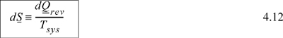
Macroscopic definition—Intensive entropy is a state property of the system. For a differential change in state of a closed simple system (no internal temperature gradients or composition gradients and no internal rigid, adiabatic, or impermeable walls),2 the differential entropy change of the system is equal to the heat absorbed by the system along a reversible path divided by the absolute temperature of the system at the surface where heat is transferred.
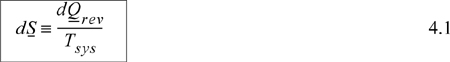
where dS is the entropy change of the system. We will later show that this definition is consistent with the microscopic definition.
Microscopic definition—Entropy is a measure of the molecular disorder of the system. Its value is related to the number of microscopic states available at a particular macroscopic state. Specifically, for a system of fixed energy and number of particles, N,
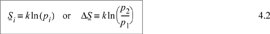
where pi is the number of microstates in the ith macrostate, k = R/NA. We define microstates and macrostates in the next section.
The microscopic perspective is directly useful for understanding how entropy changes with volume (for a gas), temperature, and mixing. It simply states that disorder increases when the number of possible arrangements increases, like the socks and drawers mentioned in the introduction. Similarly, molecules redistribute themselves when a valve is opened until the pressures have equilibrated. From the microscopic approach, entropy is a specific mathematical relation related to the number of possible arrangements of the molecule. Boltzmann showed that this microscopic definition is entirely consistent with the macroscopic property inferred by Rudolf Clausius. We will demonstrate how the approaches are equivalent.
Entropy is a difficult concept to understand, mainly because its influence on physical situations is subtle, forcing us to rely heavily on the mathematical definition. We have ways to try to make some physical connection with entropy, and we will discuss these to give you every opportunity to develop a sense of how entropy changes. Ultimately, you must reassure yourself that entropy is defined mathematically, and like enthalpy, can be used to solve problems even though our physical connection with the property is occasionally less than satisfying.
In Section 4.2, the microscopic definition of entropy is discussed. On the microscopic scale, S is influenced primarily by spatial arrangements (affected by volume and mixing), and energetic arrangements (occupation) of energy levels (affected by temperature). We clarify the meaning of the microscopic definition by analyzing spatial distributions of molecules. To make the connection between entropy and temperature, we outline how the principles of volumetric distributions extend to energetic distributions. In Section 4.3, we introduce the macroscopic definition of entropy and conclude with the second law of thermodynamics.
The second law is formulated mathematically as the entropy balance in Section 4.4. In this section we demonstrate how heat can be converted into work (as in an electrical power plant). However, the maximum thermal efficiency of the conversion of heat into work is less than 100%, as indicated by the Carnot efficiency. The thermal efficiency can be easily derived using entropy balances. This simple but fundamental limitation on the conversion of heat into work has a profound impact on energy engineering. Section 4.5 is a brief section, but makes the key point that pieces of an overall process can be reversible, even while the overall process is irreversible.
In Section 4.6 we simplify the entropy balance for common process equipment, and then use the remaining sections to demonstrate applications of system efficiency with the entropy balance. Overall, this chapter provides an understanding of entropy which is essential for Chapter 5 where entropy must be used routinely for process calculations.
4.2. The Microscopic View of Entropy
Probability theory is nothing but common sense reduced to calculation.
LaPlace
To begin, we must recognize that the disorder of a system can change in two ways. First, disorder occurs due to the physical arrangement (distribution) of atoms, and we represent this with the configurational entropy.3 There is also a distribution of kinetic energies of the particles, and we represent this with the thermal entropy. For an example of kinetic energy distributions, consider that a system of two particles, one with a kinetic energy of 3 units and the other of 1 unit, is microscopically distinct from the same system when they both have 2 units of kinetic energy, even when the configurational arrangement of atoms is the same. This second type of entropy is more difficult to implement on the microscopic scale, so we focus on the configurational entropy in this section.4
![]() Configurational entropy is associated with spatial distribution. Thermal entropy is associated with kinetic energy distribution.
Configurational entropy is associated with spatial distribution. Thermal entropy is associated with kinetic energy distribution.
Entropy and Spatial Distributions: Configurational Entropy
Given N molecules and M boxes, how can these molecules be distributed among the boxes? Is one distribution more likely than another? Consideration of these issues will clarify what is meant by microstates and macrostates and how entropy is related to disorder. Our consideration will focus on the case of distributing particles between two boxes.
![]() Distinguishability of particles is associated with microstates. Indistinguishability is associated with macrostates.
Distinguishability of particles is associated with microstates. Indistinguishability is associated with macrostates.
First, let us suppose that we distribute N = 2 ideal gas5 molecules in M = 2 boxes, and let us suppose that the molecules are labeled so that we can identify which molecule is in a particular box. We can distribute the labeled molecules in four ways, as shown in Fig. 4.1. These arrangements are called microstates because the molecules are labeled. For two molecules and two boxes, there are four possible microstates. However, a macroscopic perspective makes no distinction between which molecule is in which box. The only macroscopic characteristic that is important is how many particles are in a box, rather than which particle is in a certain box. For macrostates, we just need to keep track of how many particles are in a given box, not which particles are in a given box. It might help to think about connecting pressure gauges to the boxes. The pressure gauge could distinguish between zero, one, and two particles in a box, but could not distinguish which particles are present. Therefore, microstates α and δ are different macrostates because the distribution of particles is different; however, microstates β and γ give the same macrostate. Thus, from our four microstates, we have only three macrostates.

Figure 4.1. Illustration of configurational arrangements of two molecules in two boxes, showing the microstates. Not that β and γ would have the same macroscopic value of pressure.
To find out which arrangement of particles is most likely, we apply the “principle of equal a priori probabilities.” This “principle” states that all microstates of a given energy are equally likely. Since all of the states we are considering for our non-interacting particles are at the same energy, they are all equally likely.6 From a practical standpoint, we are interested in which macrostate is most likely. The probability of a macrostate is found by dividing the number of microstates in the given macrostate by the total number of microstates in all macrostates as shown in Table 4.1. For our example, the probability of the first macrostate is 1/4 = 0.25. The probability of the evenly distributed state is 2/4 = 0.5. That is, one-third of the macrostates possess 50% of the probability. The “most probable distribution” is the evenly distributed case.
Table 4.1. Illustration of Macrostates for Two Particles and Two Boxes

What happens when we consider more particles? It turns out that the total number of microstates for N particles in M boxes is MN, so the counting gets tedious. For five particles in two boxes, the calculations are still manageable. There will be two microstates where all the particles are in one box or the other. Let us consider the case of one particle in box A and four particles in box B. Recall that the macrostates are identified by the number of particles in a given box, not by which particles are in which box. Therefore, the five microstates for this macrostate appear as given in Table 4.2(a).
Table 4.2. Microstates for the Second and Third Macrostates for Five Particles Distributed in Two Boxes
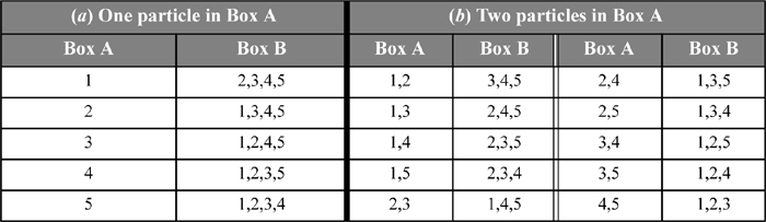
The counting of microstates for putting two particles in box A and three in box B is slightly more tedious, and is shown in Table 4.2(b). It turns out that there are 10 microstates in this macrostate. The distributions for (three particles in A) + (two in B) and for (four in A) + (one in B) are like the distributions (two in A) + (three in B), and (one in A) + (four in B), respectively. These three cases are sufficient to determine the overall probabilities. There are MN = 25 = 32 microstates total summarized in the table below.
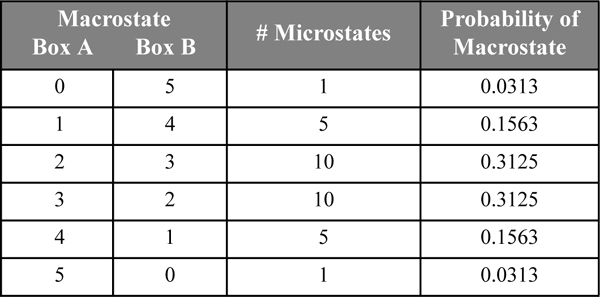
Note now that one-third of the macrostates (two out of six) possess 62.5% of the microstates. Thus, the distribution is now more peaked toward the most evenly distributed states than it was for two particles where one-third of the macrostates possessed 50% of the microstates. This is one of the most important aspects of the microscopic approach. As the number of particles increases, it won’t be long before 99% of the microstates are in one-third of the macrostates. The trend will continue, and increasing the number of particles further will quickly yield 99% of the microstates in that one-tenth of the macrostates. In the limit as N→∞ (the “thermodynamic limit”), virtually all of the microstates are in just a few of the most evenly distributed macrostates, even though the system has a very slight finite possibility that it can be found in a less evenly distributed state. Based on the discussion, and considering the microscopic definition of entropy (Eqn. 4.2), entropy is maximized at equilibrium for a system of fixed energy and total volume.7
![]() With a large number of particles, the most evenly distributed configurational state is most probable, and the probability of any other state is small.
With a large number of particles, the most evenly distributed configurational state is most probable, and the probability of any other state is small.
Generalized Microstate Formulas
To extend the procedure for counting microstates to large values of N (~1023), we cannot imagine listing all the possibilities and counting them up. It would require 40 years to simply count to 109 if we did nothing but count night and day. We must systematically analyze the probabilities as we consider configurations and develop model equations describing the process.
How do we determine the number of microstates for a given macrostate for large N? For the first step in the process, it is fairly obvious that there are N ways of moving one particle to box B, i.e., 1 came first, or 2 came first, and so on, which is what we did to create Table 4.2(a). However, counting gets more complicated when we have two particles in a box. Since there are N ways of moving the first particle to box B, and there are (N – 1) particles left, we begin with the same logic for the (N – 1) remaining particles. For example, with five particles, there would then be five ways of placing the first particle, then four ways of placing the second particle for a total of 20 possible ways of putting two particles in box B. One way of writing this would be 5·4, which is equivalent to (5·4·3·2·1)/(3·2·1), which can be generalized to N!/(N – m)!, where m is the number of particles we have placed in the first box.8 (N! is read “N factorial,” and calculated as N·(N – 1)·(N – 2)......·2·1). Our formula gives 20 ways, but Table 4.2(b) shows only 10 ways. What are we missing? Answer: When we count this way, we are implicitly double counting some microstates. Note in Table 4.2(b) that although there are two ways that we could put the first particle in box B, the order in which we place them does not matter when we count microstates. Therefore, using N!/(N – m)! implicitly distinguishes between the order in which particles are placed. For counting microstates, the history of how a particular microstate was achieved does not interest us. Therefore, we say there are only 10 distinguishable microstates.
It turns out that it is fairly simple to correct for this overcounting. For two particles in a box, they could have been placed in the order 1-2, or in the order 2-1, which gives two possibilities. For three particles, they could have been placed 1-2-3, 1-3-2, 2-1-3, 2-3-1, 3-1-2, 3-2-1, for six possibilities. For m particles in a box, without correction of the formula, we overcount by m!. Therefore, we modify the above formula by dividing by m! to correct for overcounting. Finally, the number of microstates for arranging N particles in two boxes, with m particles in one of the boxes, is:9
The general formula for M boxes is:10
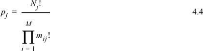
mij is the number of particles in the ith box at the jth macrostate. We will not derive this general formula, but it is a straightforward extension of the formula for two boxes which was derived above. Therefore, with 10 particles, and three in the first box, two in the second box and five in the third box, we have 10!/(3!2!5!) = 3,628,800/(6·2·120) = 2520 microstates for this macrostate.
Recall the microscopic definition of entropy given by Eqn. 4.2. Let us use it to calculate the entropy change for an ideal gas due to an isothermal change in volume. The statistics we have just derived will apply since an ideal gas consists of non-interacting particles whose energy is independent of their nearest neighbors. During an expansion like that described, the energy is constant because the system is isolated. Therefore, the temperature is also constant because dU = CV dT for an ideal gas.
Entropy and Isothermal Volume/Pressure Change for Ideal Gases
Suppose an insulated container, partitioned into two equal volumes, contains N molecules of an ideal gas in one section and no molecules in the other. When the partition is withdrawn, the molecules quickly distribute themselves uniformly throughout the total volume. How is the entropy affected? Let subscript 1 denote the initial state and subscript 2 denote the final state. Here we take for granted that the final state will be evenly distributed.
We can develop an answer by applying Eqn. 4.4, and noting that 0! = 1:
Substituting into Eqn. 4.2, and recognizing ![]() ,
,
ΔS = S2 – S1 = kln(p2/p1) = k{ln(N!) – 2 In[(N/2)!]}
Stirling’s approximation may be used for ln(N!) when N > 100,
The approximation is a mathematical simplification, and not, in itself, related to thermodynamics.
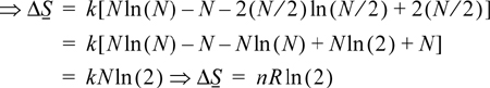
Therefore, entropy of the system has increased by a factor of ln(2) when the volume has doubled at constant T. Suppose the box initially with particles is three times as large as the empty box. In this case the increase in volume will be 33%. Then what is the entropy change? The trick is to imagine four equal size boxes, with three equally filled at the beginning.
A similar application of Stirling’s approximation gives,

We may generalize the result by noting the pattern with this result and the previous result,
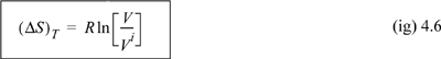
where the subscript T indicates that this equation holds at constant T. For an isothermal ideal gas, we also may express this in terms of pressure by substituting V = RT/P in Eqn. 4.6

Therefore, the entropy decreases when the pressure increases isothermally. Likewise, the entropy decreases when the volume decreases isothermally. These concepts are extremely important in developing an understanding of entropy, but by themselves, are not directly helpful in the initial objective of this chapter—that of determining inefficiencies and maximum work. The following example provides an introduction to how these conceptual points relate to our practical objectives.
Example 4.1. Entropy change and “lost work” in a gas expansion
An isothermal ideal gas expansion produces maximum work if carried out reversibly and less work if friction or other losses are present. One way of generating “other losses” is if the force of the gas on the piston is not balanced with the opposing force during the expansion, as shown in part (b) below. Consider a piston/cylinder containing one mole of nitrogen at 5 bars and 300 K is expanded isothermally to 1 bar.
a. Suppose that the expansion is reversible. How much work could be obtained and how much heat is transferred? What is the entropy change of the gas?
b. Suppose the isothermal expansion is carried out irreversibly by removing a piston stop and expanding against the atmosphere at 1 bar. Suppose that heat transfer is provided to permit this to occur isothermally. How much work is done by the gas and how much heat is transferred? What is the entropy change of the gas? How much work is lost compared to a reversible isothermal process and what percent of the reversible work is obtained (the efficiency)?
Solution
Basis: 1 mole, closed unsteady-state system.
a. The energy balance for the piston/cylinder is ΔU = Q + WEC = 0 because the gas is isothermal and ideal. dWEC = –PdV = –(nRT/V)dV; WEC = –nRTln(V2/V1) = –nRTln(P1/P2) = –(1)8.314(300)ln(5) = –4014J. By the energy balance Q = 4014J. The entropy change is by Eqn. 4.7, ΔS = –nRln(P2/P1) = –(1)8.314ln(1/5) = 13.38 J/K.
b. The energy balance does not depend on whether the work is reversible and is the same. Taking the atmosphere as the system, the work is WEC,atm = –Patm(V2,atm –V1,atm) = –WEC = –Patm(V1–V2) = Patm(nRT/P2–nRT/P1) = nRT(Patm/P2–Patm/P1) ⇒ WEC = nRT(Patm/P1–Patm/P2) = (1)8.314(300)(1/5–1) = –1995J, Q = 1995J. The entropy change depends on only the state change and this is the same as (a), 13.38 J/K. The amount of lost work is Wlost = 4014 – 1995 = 2019J, the percent of reversible work obtained (efficiency) is 1995/4014 · 100% = 49.7%.
An important point is suggested by Example 4.1, even though the example is limited to ideal gas constraints. We saw that the isothermal entropy change for the gas was the same for the reversible and irreversible changes because the gas state change was the same. Though Eqn. 4.7 is limited to ideal gases, the relation between entropy changes and state changes is generalizable as we prove later. We will show later that case (b) always generates more entropy.
Entropy of Mixing for Ideal Gases
Mixing is another important process to which we may apply the statistics that we have developed. Suppose that one mole of pure oxygen vapor and three moles of pure nitrogen vapor at the same temperature and pressure are brought into intimate contact and held in this fashion until the nitrogen and oxygen have completely mixed. The resultant vapor is a uniform, random mixture of nitrogen and oxygen molecules. Let us determine the entropy change associated with this mixing process, assuming ideal-gas behavior.
Since the Ti and Pi of both ideal gases are the same, ViN2 = 3ViO2 and Vitot = 4ViO2. Ideal gas molecules are point masses, so the presence of O2 in the N2 does not affect anything as long as the pressure is constant. The main effect is that the O2 now has a larger volume to access and so does N2. The component contributions of entropy change versus volume change can be simply added. Entropy change for O2:
ΔS = nO2Rln(4) = ntotR[–xO2ln(0.25)] = ntotR[–xO2ln(xO2)]
Entropy change for N2:
Entropy change for total fluid:
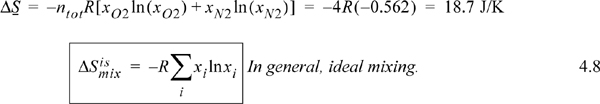
This is an important result as it gives the entropy change of mixing for non-interacting particles. Remarkably, it is also a reasonable approximation for ideal solutions where energy and total volume do not change on mixing. This equation provides the underpinning for much of the discussion of mixtures and phase equilibrium in Unit III.
The entropy of a mixed ideal gas or an ideal solution, here both denoted with a superscript “is:”

Note that these equations apply to ideal gases if we substitute y for x. In this section we have shown that a system of ideal gas molecules at equilibrium is most likely to be found in the most randomized (distributed) configuration because this is the macrostate with the largest fraction of microstates. In other words, the entropy of a state is maximized at equilibrium for a system of fixed U,V, and N.
But how can temperature be related to disorder? We consider this issue in the next subsection.
Entropy and Temperature Change: Thermal Entropy
One key to understanding the connection between thermal entropy and disorder is the appreciation that energy is quantized. Thus, there are discrete energy levels in which particles may be arranged. These energy levels are analogous to the boxes in the spatial distribution problem. The effect of increasing the temperature is to increase the energy of the molecules and make higher energy levels accessible.
To see how this affects the entropy, consider a system of three molecules and three energy levels εo, ε1 = 2εo, ε3 = 3εo. Suppose we are at a low temperature and the total energy is U = 3εo. The only way this can be achieved is by putting all three particles in the lowest energy level. The other energy levels are not accessible, and S = So. Now consider raising the temperature to give the system U = 4εo. One macrostate is possible (one molecule in ε1 and two in εo), but there are now three microstates, ΔS = kln(3). Can you show when U = 6εo that the macrostate with one particle in each level results in ΔS = kln(6)? Real systems are much larger and the molecules are more complex, but the same qualitative behavior is exhibited: increasing T increases the accessible energy levels which increases the microstates, increasing entropy.
We can advance our understanding of thermal effects on entropy by contemplating the Einstein solid.11 Albert Einstein’s (1907) proposal was that a solid could be treated as a large number of identical vibrating monatomic sites, modeling the potential energies as springs that follow Hooke’s law. The quantum mechanical analog to the energy balance is known as Shrödinger’s equation, which relates the momentum (kinetic energy) and potential energy. An exact solution is possible only for equally spaced energy levels, known as quantum levels. The equally spaced quantized states for each oscillator are separated by hf where h is Planck’s constant and f is the frequency of the oscillator. Thus, the system is described as a system of harmonic oscillators. Assuming that each oscillator and each dimension (x,y,z) is independent, we can develop an expression for the internal energy and the heat capacity.
Albert Einstein (1879 – 1955) was a German-born physicist. He contributed to an understanding of quantum behavior and the general theory of relativity. He was awarded the 1921 Nobel Prize in physics.
The Einstein solid model was one of the earliest and most convincing demonstrations of the limitations of classical mechanics. It serves today as a simple illustration of the manner in which quantum mechanics and statistical mechanics lead to consistent and experimentally verifiable descriptions of thermodynamic properties. The assumptions of the Einstein solid model are as follows:
• The total energy in a solid is the sum of M harmonic oscillator energies where M/3 is the number of atoms because the atoms oscillate independently in three dimensions. Since the energy of each oscillator is quantized, we can say that the total internal energy is
where εq is the (constant) energy step for each quantum level, and qM gives the total quantum multiplier for all oscillator quantum energies added. The term Mεq/2 represents the ground state energy that oscillators have in the lowest energy level. It is often convenient to relate the energy to the average quantum multiplier,
• Each oscillator in each dimension is independent, so we can allocate integer multiples of εq to any oscillator as long as the total sum of multipliers is qM. Each independent specification represents a microstate. For M = 3 oscillators, (3,1,1) specifies three units of energy in the first oscillator and one unit in each of the other two for a total of qM = 5, U = 5εq + 3εq/2.
• Raising the magnitude of qM (by adding heat to raise T) makes more microstates accessible, increasing the entropy.
For qM=3 units of energy distributed in an Einstein solid with M=4 oscillators, below is the detailed listing of the possible distributions of the energy, a total of 20 different distributions for three units of energy among four oscillators (a “multiplicity” of 20).

If we are trying to develop a description of a real solid with Avogadro’s number of oscillators, enumeration is clearly impractical. Fortunately, mathematical expressions for the multiplicity make the task manageable. Callen12 gives the general formula for the number of microstates as pi = (qMi+Mi–1)!/[qMi!(Mi–1)!]. There is a clever way to understand this formula. Instead of distributing qMi quanta among M oscillator “boxes,” consider that there are Mi – 1 “partitions” between oscillator “boxes.” In the table above, there are four oscillators, but there are three row boundaries. Consider that the quanta can be redistributed by all the permutations of the particles and boundaries (qMi+Mi–1)!. However, the permutations overcount in that the qMi are indistinguishable, so we divide by qMi!, and that the (Mi–1) boundaries are indistinguishable, so we divide by (Mi–1)!. To apply the formula for qM=2, M=2:
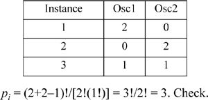
For the case with qM = 3 and M = 4, pi = (3+4–1)!/[3!(3!)] = 20, as enumerated above.
Example 4.2. Stirling’s approximation in the Einstein solid
a. Show that Callen’s formula is consistent with enumeration for:
1. qM = 3, M = 3; (2) qM = 4, M = 3
b. Use the general formula to develop an expression for S = S(qM,M) when M > 100. Express the answer in terms of the average quantum multiplier, <qM>.
c. Plot S/Mk versus <qM>. What does this indicate about entropy changes when heat is added?
Solution
a.
1. (3,0,0),(0,3,0),(0,0,3),(2,1,0),(2,0,1),(1,2,0),(1,0,2),(0,2,1),(0,1,2),(1,1,1) = 10. Check.
2. (4,0,0), (0,4,0), (0,0,4), (3,1,0), (3,0,1), (1,3,0), (1,0,3), (0,3,1), (0,1,3), (2,1,1), (1,2,1), (1,1,2), (2,0,2), (2,2,0), (0,2,2) = 15. Check.
b. Si = k ln(pi) = k { ln[(qMi+Mi–1)!] – ln[qMi!(Mi–1)!] }. Applying Stirling’s approximation,
S/k = [(qM+M–1)ln(qM+M–1)–(qM+M–1)] – qMlnqM + qM – (M–1)ln(M–1) + M–1 = S/Mk = (qM/M)ln[(qM+M–1)/qM] + [(M–1)/M]ln[(qM+M–1)/(M–1)]
S/Mk = <qM>ln(1+1/<qM>) + ln(<qM>+1)
c. Fig. 4.2 shows that S increases with <qM> = qM/M (=U/Mεq – ½). When T increases, U will increase, meaning that <qM> and S increase. It would be nice to relate the change in entropy quantitatively to the change in temperature, but a complete analysis of the entire temperature range requires advanced derivative manipulations that distracts from the main concepts at this stage. We return to this problem in Chapter 6.
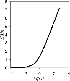
Figure 4.2. Entropy of the Einstein solid with increasing energy and T as explained in Example 4.2.
You should notice that we represented the interactions of the monatomic sites as if they were connected by Hooke’s law springs in the solid phase. They are not rigorously connected this way, but the simple model approximates the behavior of two interacting molecules in a potential energy well. If the spring analogy were exact, the potential energy well would be a parabola (thus a harmonic oscillator). Look back at the Lennard-Jones potential in Chapter 1 and you can see that the shape is a good approximation if the atoms do not vibrate too far from the minimum in the well. The Einstein model gives qualitatively the right behavior, but the Debye model that followed in 1912 is more accurate because it represents collective waves moving through the solid. We omit discussion of the Debye model because our objectives are met with the Einstein model.13 We briefly extend the concept of the Einstein model in Chapter 6 where we develop more powerful methods for manipulation of derivatives.
In the present day, the subtle relations between entropy and molecular distributions are complex but approachable. Imagine how difficult gaining this understanding must have been for Boltzmann in 1880, before the advent of quantum mechanics. Many scientists at the time refused even to accept the existence of molecules. Trying to explain to people the nature and significance of his discoveries must have been extremely frustrating. What we know for sure is that Boltzmann drowned himself in 1903. Try not to take your frustrations with entropy quite so seriously.
Test Yourself
1. Does molar entropy increase, decrease, or stay about the same for an ideal gas if: (a) volume increases isothermally?; (b) pressure increases isothermally?; (c) temperature increases isobarically?; (d) the gas at the vapor pressure condenses?; (e) two pure gas species are mixed?
2. Does molar entropy increase, decrease, or stay about the same for a liquid if: (a) temperature increases isobarically?; (b) pressure increases isothermally?; (c) the liquid evaporates at the vapor pressure?; (d) two pure liquid species are mixed?
4.3. The Macroscopic View of Entropy
In the introduction to this chapter, we alluded to the relation between entropy and maximum process efficiency. We have shown that entropy changes with volume (pressure) and temperature. How can we use entropy to help us determine maximum work output or minimum work input? The answer is best summarized by a series of statements. These statements refer to the entropy of the universe. This does not mean that we imagine measuring entropy all over the universe. It simply means that entropy may decrease in one part of a system but then it must increase at least as much in another part of a system. In assessing the reversibility of the overall system, we must sum all changes for each process in the overall system and its surroundings. This is the relevant part of the universe for our purposes.
Molar or specific entropy is a state property which will assist us in the following ways.
1. Irreversible processes will result in an increase in entropy of the universe. (Irreversible processes will result in entropy generation.) Irreversible processes result in loss of capability for performing work.
2. Reversible processes result in no increase in entropy of the universe. (Reversible processes result in zero entropy generation. This principle will be useful for calculation of maximum work output or minimum work input for a process.)
3. Proposed processes which would result in a decrease of entropy of the universe are impossible. (Impossible processes result in negative entropy generation.)
These three principles are summarized in the second law of thermodynamics: Reversible processes and/or optimum work interactions occur without entropy generation, and irreversible processes result in entropy generation. The microscopic descriptions in the previous section teach us very effectively about the relation between entropy and disorder, but it is not fair to say that any increase in volume results in a loss of potentially useful work when the entropy of the system increases. (Note that it is the entropy change of the universe that determines irreversibility, not the entropy change of the system.) After all, the only way of obtaining any expansion/contraction work is by a change in volume. To understand the relation between lost work and volume change, we must appreciate the meaning of reversibility, and what types of phenomena are associated with entropy generation. We will explore these concepts in the next sections.
Entropy Definition (Macroscopic)
Let us define the differential change in entropy of a closed simple system by the following equation:
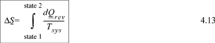
For a change in states, both sides of Eqn. 4.12 may be integrated,
where the following occurs:
1. The entropy change on the left-hand side of Eqn. 4.13 is dependent only on states 1 and 2 and not dependent on reversibility. However, to calculate the entropy change via the integral, the integral may be evaluated along any convenient reversible pathway between the actual states.
2. Tsys is the temperature of the system boundary where heat is transferred. Only if the system boundary temperature is constant along the pathway may this term be taken out of the integral sign.
A change in entropy is completely characterized for a pure single-phase fluid by any other two state variables. It may be surprising that the integral is independent of the path since Q is a path-dependent property. The key is to understand that the right-hand side integral is independent of the path, as long as the path is reversible. Thus, a process between two states does not need to be reversible to permit calculation of the entropy change, since we can evaluate it along any reversible path of choice. If the actual path is reversible, then the actual heat transfer and pathway may be used. If the process is irreversible, then any reversible path may be constructed for the calculation.
![]() Entropy is a state property. For a pure single-phase fluid, specific entropy is characterized by two state variables (e.g., T and P).
Entropy is a state property. For a pure single-phase fluid, specific entropy is characterized by two state variables (e.g., T and P).
Look back at Example 4.1 and note that the entropy change for the isothermal process was calculated by the microscopic formula. However, look at the process again from the perspective of Eqn. 4.13 and subsequent statement 2. Because the process was isothermal, the entropy change can be calculated ΔS = Qrev/Tsys; try it! Note that the irreversible process in that example exhibits the same entropy change, calculated by the reversible pathway.
Now, look back at the integral of Eqn. 4.13 and consider an adiabatic, reversible process; the process will be isentropic (constant entropy, ΔS = 0). Let us consider how the entropy can be used as a state property to identify the final state along a reversible adiabatic process. Further, the property does not depend on the limitations of the ideal gas law. The ideal gas law was convenient to introduce the property. Consider the adiabatic reversible expansion of steam, a non-ideal gas. We can read S values from the steam tables.
Example 4.3. Adiabatic, reversible expansion of steam
Steam is held at 450°C and 4.5 MPa in a piston/cylinder. The piston is adiabatically and reversibly expanded to 2.0 MPa. What is the final temperature? How much reversible work can be done?
Solution
The T, P are known in the initial state, and the value of S can be found in the steam tables. Steam is not an ideal gas, but by Eqn. 4.12, the process is isentropic because it is reversible and adiabatic. From the steam tables, the entropy at the initial state is 6.877 kJ/kgK. At 2 MPa, this entropy will be found between 300°C and 350°C. Interpolating,
The P and Sf = Si are known in the final state and these two state properties can be used to find all the other final state properties. The work is determined by the energy balance: ΔU = Q + WEC. The initial value of U is 3005.8 kJ/kg. For the final state, interpolating U by using Sf at Pf, U = 2773.2 + 0.572(2860.5 – 2773.2) = 2823.1 kJ/kg, so
WEC = (2823.1 – 3005.8) = –182.7 kJ/kg
Let us revisit the Carnot cycle of Section 3.1 in light of this new state property, entropy. The Carnot cycle was developed with an ideal gas, but it is possible to prove that the cycle depends only on the combination of two isothermal steps and two adiabatic steps, not the ideal gas as the working fluid.14 Because the process is cyclic, the final state and initial state are identical, so the overall entropy changes of the four steps must sum to zero, ΔS = 0. Because the reversible, adiabatic steps are isentropic, ΔS = 0, the entropy change for the two isothermal steps must sum to zero. As we discussed above, for an isothermal step Eqn. 4.13 becomes ΔS = Qrev/T. Therefore, an analysis of the Carnot cycle from the viewpoint of entropy is

This can be inserted into the formula for Carnot efficiency, Eqn. 3.6. Note that this relation is not constrained to an ideal gas! In fact, there are only three constraints for this balance: The process is cyclic; all heat is absorbed at TH; all heat is rejected at TC. Example 4.4 shows how the Carnot cycle can be performed with steam including phase transformations.
Example 4.4. A Carnot cycle based on steam
Fig. 4.3 shows the path of a Carnot cycle operating on steam in a continuous cycle that parallel the two isothermal steps and two adiabatic steps of Section 3.1. First, saturated liquid at 5 MPa is boiled isothermally to saturated vapor in step (a→b). In step (b→c), steam is adiabatically and reversibly expanded from saturated vapor at 5 MPa to 1 MPa. In (c→d), heat is isothermally removed and the volume drops during condensation. Finally, in step (d→a), the steam is adiabatically and reversibly compressed to 5 MPa and saturated liquid. (Hint: Challenge yourself to solve the cycle without looking at the solution.).
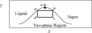
Figure 4.3. A T-S diagram illustrating a Carnot cycle based on steam.
a. Compute W(a→b) and QH.
b. Compute W(b→c).
c. Compute W(d→a). (The last step in the cycle).
d. Compute W(c→d) and QC. (The third step in the cycle).
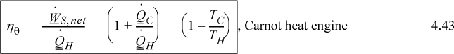
e. For the cycle, compute the thermal efficiency by ηθ = –Wnet/QH and compare to Carnot’s efficiency, ηθ = (TH – TL)/TH.
Solution
The entropy change is zero for the expansion and compression steps because these steps are adiabatic and reversible, as indicated by the vertical line segments in Fig. 4.3.
a. E-balance: fixed P,T vaporization, QH = ΔU – WEC = (ΔU + PΔV) = ΔHvap = 1639.57 J/kg; WEC(a→b) = PΔV = 5(0.0394 – 0.001186)*1000 = 191.1 J/kg.
b. E-balance: isentropic, WEC(b→c) = ΔU; Ub = U(sat. vap., 5MPa) = 2596.98 kJ/kg; S-balance: ΔS = 0; Sc = Sb = 5.9737 kJ/kg-K= qc(6.5850) + (1 – qc)2.1381; qc = 0.8625; Uc = 0.8625(2582.75) + (1 – 0.8625)761.39 = 2332.31 kJ/kg; WEC(b→c) = 2332.31 – 2596.98 = –264.67 kJ/kg.
c. This is the last step. E-balance: isentropic. WEC(d→a) = ΔU; Ud = U(sat. liq., 5MPa) = 1148.21 kJ/kg; the quality at state d is not known, but we can use the entropy at state a to find it. S-balance: ΔS = 0; Sd = Sa = 2.9210 kJ/kg-K= qd(6.5850) + (1 – qd)2.1381; qd = 0.1761; Ud = 0.1761(2582.75) + (1 – 0.1761)761.39 = 1082.13 kJ/kg; WEC(d→a) = 1082.13 – 1148.21 = –66.08 kJ/kg.
d. This is the third step using the quality for d calculated in part (c). This is a fixed T,P condensation. E-balance: QC = ΔU – WEC = (ΔU+PΔV) = ΔH; Hd = 762.52 + 0.1761(2014.59) = 1117.29 kJ/kg; Hc= 762.52 + 0.8625(2014.59) = 2500.10 kJ/kg; QC = Hd – Hc = –1382.21 kJ/kg WEC = PΔV; Vc = 0.001127(1 – 0.8625) + 0.8625(0.1944) = 0.1678 m3/kg = 167.8 cm3/g Vd = 0.001127(1 – 0.1761)+0.1761(0.1944) = 0.0352 m3/kg = 35.2 cm3/g W(c→d) = 1.0(35.2 – 167.8) = –132.6 MPa-cm3/g = –132.6 kJ/kg
e. ηθ = –Wnet/QH; Wnet = (264.67–66.08+191.1–132.6) = 257.1 kJ/kg; ηθ = 257.1/1639.57 = 0.157; ηθ (Carnot) = (263.94–179.88)/(263.94+273.15) = 0.157. The actual cycle matches the Carnot formula. Note that the cyclic nature of this process means that we could have computed more quickly by Wnet = –(QC + QH) = 1382.21 – 1639.57 = 257.4 kJ/kg.
The macroscopic view of entropy can be bewildering when first studied because students strive to understand the physical connection. The microscopic view of entropy is helpful for some students but a significant disconnect often persists. In either case, if you review the definitions at the beginning of the chapter, both are mathematical, not physical. In Chapter 2 we discussed that Q was a path-dependent property, but now we are demonstrating that dividing the quantity by T and integrating along a path results in a quantity that is independent of the path!15 Some students find it helpful to accept this as a mathematical relationship with the name of “entropy.” In fact, development of the macroscopic definition of entropy was not obvious to the scientists who eventually proved it to be a state property. The scientific literature at the time of Carnot can be confusing to read because the realization of the state nature of the integral was not obvious, but was developed by a significant amount of diligence and insight by the scientists of the day.
Note that entropy does not depend directly on the work done on a system. Therefore, it may be used to decouple heat and work in the energy balance for reversible processes. Also for reversible processes, entropy provides a second property that may be used to determine unknowns in a process as we have seen in the previous two examples. In fact, the power of this property is that it can be used to evaluate reversibility of processes, and such understanding is critical as we search sustainable energy management practices, such as CO2 sequestration. Let us investigate some convenient pathways for the evaluation of entropy changes before we develop examples that utilize the pathways.
Calculation of Entropy Changes in Closed Systems
As with enthalpy and internal energy, tables and charts are useful sources for entropy information for common fluids. Note the tabulation of S in the tables of Appendix E. These tables and charts are calculated using the definition of entropy and procedures for non-ideal fluids that we will discuss in upcoming chapters.
For manual calculations of entropy, we develop some simple procedures here, and more rigorous procedures in Chapter 8. Since the integral of Eqn. 4.13 must be evaluated along a reversible path, let us consider some easy choices for paths. For a closed reversible system without shaft work, the energy balance in Eqn. 2.16 becomes,

Inserting Eqn. 2.3,
We now consider how this equation may be substituted in the integral of Eqn. 4.13 for calculating entropy changes in several situations.
Constant Pressure (Isobaric) Pathway
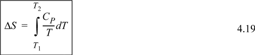
Many process calculations involve state changes at constant pressure. Recognizing H = U + PV, dH = dU + PdV + VdP. In the case at hand, dP happens to be zero; therefore, Eqn. 4.16 becomes
Since dH = CPdT at constant pressure, along a constant-pressure pathway, substituting for dQrev in Eqn. 4.13, the entropy change is
Constant Volume Pathway
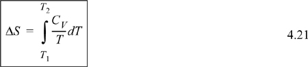
For a constant volume pathway, Eqn. 4.16 becomes
Since dU = CVdT along a constant volume pathway, substituting for dQrev in Eqn. 4.13, the entropy change is
Constant Temperature (Isothermal) Pathway
The behavior of entropy at constant temperature is more difficult to generalize in the absence of charts and tables because dQrev depends on the state of aggregation. For the ideal gas, dU = 0 = dQ – PdV, dQ = RTdV/V, and plugging into Eqn. 4.13,

For a liquid or solid, the effect of isothermal pressure of volume change is small as a first approximation; the precise relations for detailed calculations will be developed in Chapters 6–8. Looking at the steam tables at constant temperature, entropy is very weakly dependent on pressure for liquid water. This result may be generalized to other liquids below Tr = 0.75 and also to solids. For condensed phases, to a first approximation, entropy can be assumed to be independent of pressure (or volume) at fixed temperature.
Adiabatic Pathway
A process that is adiabatic and reversible will result in an isentropic path. By Eqn. 4.13,

Note that a path that is adiabatic, but not reversible, will not be isentropic. This is because a reversible adiabatic process starting at the same state 1 will not follow the same path, so it will not end at state 2, and reversible heat transfer will be necessary to reach state 2.
Phase Transitions
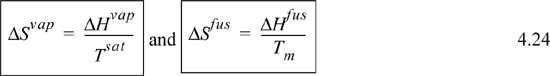
In the absence of property charts or tables, entropy changes due to phase transitions can be easily calculated. Since equilibrium phase transitions for pure substances occur at constant temperature and pressure, for vaporization
where Tsat is the equilibrium saturation temperature. Likewise for a solid-liquid transition,
where Tm is the equilibrium melting temperature. Since either transition occurs at constant pressure if along a reversible pathway, we may include Eqn. 4.17, giving
Now let us examine a process from Chapter 2 that was reversible, and study the entropy change. We will show that the result is the same via two different paths, confirming that entropy is a state function.
Example 4.5. Ideal gas entropy changes in an adiabatic, reversible expansion
In Example 2.11 on page 75, we derived the temperature change for a closed-system adiabatic expansion of an ideal gas. How does the entropy change along this pathway, and what does this example show about changes in entropy with respect to temperature?
Solution
Reexamine the equation (CV/T)dT = –(R/V)dV, which may also be written (CV/R)dln T = –dIn V. We can sketch this path as shown by the diagonal line in Fig. 4.4. Since our path is adiabatic (dQ = 0) and reversible, and our definition of entropy is dS = (dQrev)/T, we expect that this implies that the path is also isentropic (a constant-entropy path). Since entropy is a state property, we can verify this by calculating entropy along the other pathway of the figure consisting of a constant temperature (step A) and a constant volume (step B)
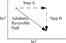
Figure 4.4. Equivalence of an adiabatic and an alternate path on a T-V diagram.
For the reversible isothermal step we have
Thus,
Substituting the ideal gas law,
For the constant volume step, we have
dU = dQrev or CVdT = dQrev
Thus,
We could replace a differential step along the adiabat (adiabatic pathway) with the equivalent differential steps along the alternate pathways; therefore, we can see that the change in entropy is zero,
which was shown by the energy balance in Eqn. 2.62, and we verify that the overall expansion is isentropic. Trials with additional pathways would show that ΔS is the same.
![]() The entropy change along the adiabatic, reversible path is the same as along (step A + step B) illustrating that S is a state property.
The entropy change along the adiabatic, reversible path is the same as along (step A + step B) illustrating that S is a state property.
The method of subdividing state changes into individual temperature and volume changes can be generalized to any process, not just the adiabatic process of the previous example, giving

We may integrate steps A and B independently. We also could use temperature and pressure steps to calculate entropy changes, resulting in an alternate formula:
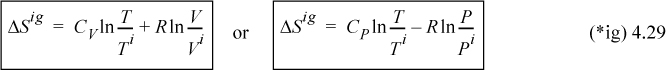
As an exercise, you may wish to choose two states and find the change in S along two different pathways: first with a step in T and then in P, and then by inverting the steps. The heat and work will be different along the two paths, but the change in entropy will be the same.
Looking back at Eqn. 4.26, we realize that it does not depend on the ideal gas assumption, and it is a general result,
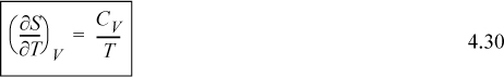
which provides a relationship between CV and entropy. Similarly, looking back at Eqn. 4.18,

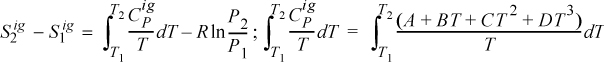
Eqns. 4.30 and 4.31 are particularly easy to apply for ideal gases. In fact, the most common method for evaluating entropy changes with temperature applies Eqn. 4.31 in this way, as shown below.
Example 4.6. Ideal gas entropy change: Integrating CPig(T)
Propane gas undergoes a change of state from an initial condition of 5 bar and 105°C to 25 bar and 190°C. Compute the change in enthalpy using the ideal gas law.
Solution
Because P and T are specified in each state, the ideal gas change is calculated most easily by combining an isobaric temperature step, Eqns. 4.19, and an isothermal pressure change, Eqn. 4.22. The heat capacity constants are obtained from Appendix E.

Entropy Generation
At the beginning of Section 4.3 on page 142, statement number one declares that irreversible processes generate entropy. Now that some methods for calculating entropy have been presented, this principle can be explored.
Example 4.7. Entropy generation and “lost work”
In Example 4.1 consider the surroundings at 300 K: (a) Consider the entropy change in the surroundings and the universe for parts 4.1(a) and 4.1(b) and comment on the connection between entropy generation and lost work; (b) How would entropy generation be affected if the surroundings are at 310 K?
a. For 4.1(a) the entropy change of the surroundings is ![]() . This is equal and opposite to the entropy change of the piston/cylinder, so the overall entropy change is ΔSuniverse = 0.
. This is equal and opposite to the entropy change of the piston/cylinder, so the overall entropy change is ΔSuniverse = 0.
For part 4.1(b), the entropy change of the universe is ΔSsurr = Q/300 = –1995/300 = –6.65J/K. The total entropy change is ΔSuniverse = 13.38–6.65 = 6.73J/K > 0, thus entropy is generated when work is lost.
b. If the temperature of the surroundings is raised to 310K, then for the reversible piston cylinder expansion for 4.1(a), ΔSsurr = –4014/310 = –12.948J/K, and ΔSuniverse = 13.38 – 12.95 = 0.43J/K > 0. This process now will have some ‘lost work’ due to the temperature difference at the boundary even though the piston/cylinder and work was frictionless without other losses. We will reexamine heat transfer in a gradient in a later example. For case 4.1(b), the entropy generation is still greater, indicating more lost work, ΔSsurr = –1995/310 = –6.43J/K, ΔSuniverse = 13.38 – 6.43 = 6.95J/K > 0.
Note: When the entropy change for the universe is positive the process is irreversible. Because entropy is a state property, the integrals that we calculate may be along any reversible pathway, and the time dependence along that pathway is unimportant.
We discussed in Chapter 2 that friction and velocity gradients result in irreversibilities and thus entropy generation occurs. Entropy generation can also occur during heat transfer, so let us consider that possibility.
Example 4.8. Entropy generation in a temperature gradient
A 500 mL glass of chilled water at 283 K is removed from a refrigerator. It slowly equilibrates to room temperature at 298 K. The process occurs at 1 bar. Calculate the entropy change of the water, ΔSwater, the entropy change of the surroundings, ΔSsurr, and the entropy change of the universe, ΔSuniv. Neglect the heat capacity of the container. For liquid water CP = 4.184 J/g-K.
Solution
Water: The system is closed at constant pressure with Ti = 283 K and Tf = 298 K. We choose any reversible pathway along which to evaluate Eqn. 4.13, a convenient path being constant-pressure heating. Thus,
dQrev = dH = mCPdT
Substituting this into our definition for a change in entropy, and assuming a T-independent CP,
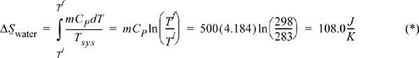
Surroundings: The surroundings also undergo a constant pressure process as a closed system; however, the heat transfer from the glass causes no change in temperature—the surroundings act as a reservoir and the temperature is 298 K throughout the process. The heat transfer of the surroundings is the negative of the heat transfer of the water, so we have

Note that the temperature of the surroundings was constant, which simplified the integration.
Universe: For the universe we sum the entropy changes of the two subsystems that we have defined. Summing the entropy change for the water and the surroundings we have
Entropy has been generated. The process is irreversible.
4.4. The Entropy Balance
In Chapter 2 we used the energy balance to track energy changes of the system by the three types of interactions with the surroundings—flow, heat, and work. This method was extremely helpful because we could use the balance as a checklist to account for all interactions. Therefore, we present a general entropy balance in the same manner. To solve a process problem we can use an analogous balance approach of starting with an equation including all the possible contributions that might occur and eliminating the balance terms that do not apply for the situation under consideration.
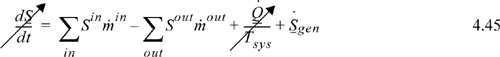
Entropy change within a system boundary will be given by the difference between entropy which is transported in and out, plus entropy changes due to the heat flow across the boundaries, and in addition, since entropy may be generated by an irreversible process, an additional term for entropy generation is added. A general entropy balance is
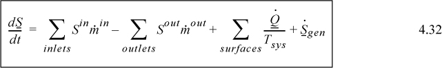
Like the energy balance, the quantity to the left of the equals sign represents the entropy change of the system. The term representing heat transfer should be applied at each location where heat is transferred and the Tsys for each term is the system temperature at each boundary where the heat transfer occurs. The heat transfer represented in the general entropy balance is the heat transfer which occurs in the actual process. We may simplify the balance for steady-state or closed systems:
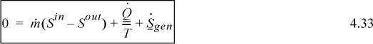

The heat flow term(s) are always written in the balance with a “plus” from the perspective of the system for which the balance is written.
The entropy balance provides us with an additional equation which may be used in solving thermodynamic problems; however, in irreversible processes, the entropy generation term usually cannot be calculated from first principles. Thus, it is an unknown in Eqns. 4.32–4.34. The balance equation is not useful for calculating any other unknowns when Sgen is unknown. In Example 4.8 the problem would have been difficult if we applied the entropy balance to the water or the surroundings independently, because we did not know how to calculate Sgen for each subsystem. However, we could calculate ΔS for each subsystem along reversible pathways. Summing the entropy changes for the subsystems of the universe, we obtain the entropy change of the universe. Consider the right-hand side of the entropy balance when written for the universe in this example. There is no mass flow in and out of the universe—it all occurs between the subsystems of the universe. In addition, heat flow also occurs between subsystems of the universe, and the first three terms on the right-hand side of the entropy balance are zero. Therefore, the entropy change of the universe is equal to the entropy generated in the universe.
The criterion for the feasibility of a process is that the entropy generation term must be greater than or equal to zero. The feasibility may not be determined unequivocally by ΔS for the system unless the system is the universe.
Note: As we work examples for irreversible processes, note that we do not apply the entropy balance to find entropy changes. We always calculate entropy changes by alternative reversible pathways that reach the same states, then we apply the entropy balance to find how much entropy was generated.
Alternatively, for reversible processes, we do apply the entropy balance because we set the entropy generation term to zero.
Let us now apply the entropy balance—first to another heat conduction problem. In Example 4.8 we studied an unsteady-state system. Now let us consider steady-state heat transfer to show which entropy balance terms are important in this application. In this example, we show that such heat conduction results in entropy generation because entropy generation occurs where the temperature gradient exists.
Example 4.9. Entropy balances for steady-state composite systems
Imagine heat transfer occurring between two reservoirs.
a. A steady-state temperature profile for such a system is illustrated in Fig. (a) below. (Note that the process is an unsteady state with respect to the reservoirs, but the focus of the analysis here is on the wall.) The entire temperature gradient occurs within the wall. In this ideal case, there is no temperature gradient within either reservoir (therefore, the reservoirs are not a source of entropy generation). Note that the wall is at steady state. Derive the relevant energy and entropy balances, carefully analyzing three subsystems: the hot reservoir, the cold reservoir, and the wall. Note that a superficial view of the reservoirs and wall is shown in Fig. (b).
b. Suppose the wall was replaced by a reversible Carnot engine across the same reservoirs, as illustrated in Fig. (c). Combine the energy and entropy balances to obtain the thermal efficiency.
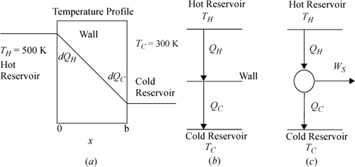
Note: Keeping track of signs and variables can be confusing when the universe is divided into multiple subsystems. Heat flow on the hot side of the wall will be negative for the hot reservoir, but positive for the wall. Since the focus of the problem is on the wall or the engine, we will write all symbols from the perspective of the wall or engine and relate to the reservoirs using negative signs and subscripts.
Solution
a. Since the wall is at steady state, the energy balance for the wall shows that the heat flows in and out are equal and opposite:
The entropy balance in each reservoir simplifies:

The entropy generation term drops out because there is no temperature gradient in the reservoirs. Taking the hot reservoir as the subsystem and noting that we have defined QH and QC to be based on the wall, we write:

where the heat fluxes are equated by the energy balance.
Now consider the entropy balance for the wall subsystem. Entropy is a state property, and since no state properties throughout the wall are changing with time, entropy of the wall is constant, and the left-hand side of the entropy balance is equal to zero. Note that the entropy generation term is kept because we know there is a temperature gradient:
Noting the relation between the heat flows in Eqn. 4.35, we may then write for the wall:
Then the wall with the temperature gradient is a source of entropy generation. Summarizing,

Hence we see that the wall is the source of entropy generation of the universe, which is positive. Notice that inclusion of the wall is important in accounting for the entropy generation by the entropy balance equations.
b. The overall energy balance relative for the engine is:

The the engine operates a steady-state cycle, dSengine/dt = 0 (it is internally reversible):

As before, ![]() and we have derived it using the entropy balance. Note that the heat flows are no longer equal and are such that the entropy changes of the reservoirs sum to zero.
and we have derived it using the entropy balance. Note that the heat flows are no longer equal and are such that the entropy changes of the reservoirs sum to zero.
We have concluded that heat transfer in a gradient results in entropy production. How can we transfer heat reversibly? If the size of the gradient is decreased, the right-hand side of Eqn. 4.37 decreases in magnitude; coincidentally, heat conduction slows, through the following relation:16
A smaller temperature gradient decreases the rate of production of entropy, but from a practical standpoint, it requires a longer time to transfer a fixed amount of heat. If we wish to transfer heat reversibly from two reservoirs at finitely different temperatures, we must use a heat engine, as described in part (b). In addition to transferring the heat reversibly, use of a heat engine generates work.
Summary: This example has shown that boundaries (walls) between systems can generate entropy. In this example, entropy was not generated in either reservoir because no temperature profile existed. The entropy generation occurred within the wall.
Note that we could have written the engine work of part (b) as follows:
Compare this to Eqn. 4.37, the result of the steady-state entropy generation. If we run the heat transfer process without obtaining work, then the universe loses a quantity of work equal to the following:
Note that TC, the colder temperature of our engine, is important in relating the entropy generation to the lost work. TC can be called the temperature at which the work is lost. Lost work is explored more completely in Section 4.12. Also note that we have chosen to operate the heat engine at temperatures which match the reservoir temperatures. This is arbitrary, but is required to obtain the maximum amount of work. The heat engine may be reversible without this constraint, but the entire process will not be reversible. These details are clarified in the next section.
An entirely analogous analysis of heat transfer would apply if we ran the heat engine in reverse, as a heat pump. Only the signs would change on the direction the heat and work were flowing relative to the heat pump. Therefore, the use of entropy permits us to reiterate the Carnot formulas in the context of all fluids, not just ideal gases.
4.5. Internal Reversibility
A process may be irreversible due to interactions at the boundaries (such as discussed in Example 4.9 on page 155) even when each system in the process is reversible. Such a process is called internally reversible. Such a system has no entropy generation inside the system boundaries. We have derived equations for Carnot engines and heat pumps, assuming that the devices operate between temperatures that match the reservoir temperatures. While such restrictions are not necessary for internal reversibility, we show here that the work is maximized in a Carnot engine at these conditions and minimized in a Carnot heat pump. Note that in development of the Carnot devices, the only temperatures of concern are the operating temperatures at the hot and cold portions of the cycle. In the following illustrations, the internally reversible engine or pump operates between TH and TC, and the reservoir temperatures are T2 and T1.
Heat Engine
A schematic for a Carnot engine is shown in Fig 4.5(a). Heat is being transferred from the reservoir at T2 to the reservoir at T1, and work is being obtained as a result. In order for heat transfer to occur between the reservoirs and the heat engine in the desired direction, we must satisfy T2 ≥ TH >TC≥T1, and since the thermal efficiency is given by Eqn. 3.6, for maximum efficiency (maximum work), TC should be as low as possible and TH as high as possible, i.e., set TH = T2, TC = T1.

Figure 4.5. Schematic of a heat engine (a) and heat pump (b). The temperatures of the reservoirs are not required to match the reversible engine temperatures, but work is optimized if they do, as discussed in the text.
![]() The operating temperatures of a reversible heat engine or heat pump are not necessarily equal to the surrounding’s temperatures; however, the optimum work interactions occur if they match the surrounding’s temperature because matching the temperatures eliminates the finite temperature-driving force that generates entropy.
The operating temperatures of a reversible heat engine or heat pump are not necessarily equal to the surrounding’s temperatures; however, the optimum work interactions occur if they match the surrounding’s temperature because matching the temperatures eliminates the finite temperature-driving force that generates entropy.
Heat Pump
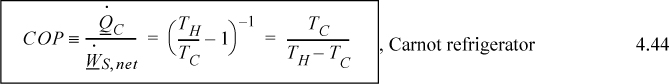
A schematic for a Carnot heat pump is shown in Fig. 4.5(b). Heat is being transferred from a reservoir at T1 to the reservoir at T2, and work is being supplied to achieve the transfer. In order for heat transfer to occur between the reservoirs and the heat engine in the desired direction, we must satisfy T2 ≤ TH > TC ≤ T1. Since the COP is given by Eqn. 4.44, for maximum COP (minimum work), TC should be as high as possible and TH as low as possible, i.e., set TC = T1, TH = T2. Therefore, optimum work interactions occur when the Carnot device operating temperatures match the surrounding temperatures. We use this feature in future calculations without special notice.
4.6. Entropy Balances for Process Equipment
Before analysis involving multiple process units, it is helpful to consider the entropy balance for common steady-state process equipment. Familiarity with these common units will facilitate rapid analysis of situations with multiple units, because understanding these balances is a key step for the calculation of reversible heat and work interactions.
Simple Closed Systems
Changes in entropy affect all kinds of systems. We have previously worked with piston/cylinders and even a glass of water. You should be ready to adapt the entropy balance in creative ways to everyday occurrences as well as sophisticated equipment.
Example 4.10. Entropy generation by quenching
A carbon-steel engine casting [CP = 0.5 kJ/kg°C] weighing 100 kg and having a temperature of 700 K is heat-treated to control hardness by quenching in 300 kg of oil [CP = 2.5 kJ/kg°C] initially at 298 K. If there are no heat losses from the system, what is the change in entropy of: (a) the casting; (b) the oil; (c) both considered together; and (d) is this process reversible?
Solution
Unlike the previous examples, there are no reservoirs, and the casting and oil will both change temperature. The final temperature of the oil and the steel casting is found by an energy balance. Let Tf be the final temperature in K.
Energy balance: The total change in energy of the oil and steel is zero.
Heat lost by casting:
Q = mCpΔT = 100 (0.5) (700 – Tf)
Heat gained by oil:
Q = mCpΔT = 300 (2.5) (Tf – 298) ⇒ balancing the heat flow, Tf = 323.1 K
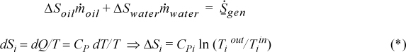
Entropy balance: The entropy change of the universe will be the sum of the entropy changes of the oil and casting. We will not use the entropy balance directly except to note that ΔSuniv = Sgen. We can calculate the change of entropy of the casting and oil by any reversible pathway which begins and ends at the same states. Consider an isobaric path:
a. Change in entropy of the casting:
b. Change in entropy of the oil (the oil bath is of finite size and will change temperature as heat is transferred to it):
c. Total entropy change: Sgen = ΔSuniv = 60.65 – 38.7 = 21.9 kJ/K
d. Sgen > 0; therefore irreversible; compare the principles with Example 4.8 on page 152 to note the similarities. The difference is that both subsystems changed temperature.
Heat Exchangers
The entropy balance for a standard two-stream heat exchanger is given by Eqn. 4.45. Since the unit is at steady state, the left-hand side is zero. Applying the entropy balance around the entire heat exchanger, there is no heat transfer across the system boundaries (in the absence of heat loss), so the heat-transfer term is eliminated. Since heat exchangers operate by conducting heat across tubing walls with finite temperature driving forces, we would expect the devices to be irreversible. Indeed, if the inlet and outlet states are known, the flow terms may be evaluated, thus permitting calculation of entropy generation.
We also may perform “paper” design of ideal heat transfer devices that operate reversibly. If we set the entropy generation term equal to zero, we find that the inlet and outlet states are constrained. Since there are multiple streams, the temperature changes of the streams are coupled to satisfy the entropy balance. In order to construct such a reversible heat transfer device, the unit would need to be impracticably large to only have small temperature gradients.
Example 4.11. Entropy in a heat exchanger
A heat exchanger for cooling a hot hydrocarbon liquid uses 10 kg/min of cooling H2O which enters the exchanger at 25°C. Five kg/min of hot oil enters at 300°C and leaves at 150°C and has an average specific heat of 2.51 kJ/kg-K.
a. Demonstrate that the process is irreversible as it operates now.
b. Assuming no heat losses from the unit, calculate the maximum work which could be obtained if we replaced the heat exchanger with a Carnot device which eliminates the water stream and transfers heat to the surroundings at 25°C

Solution
a. System is heat exchanger (open system in steady-state flow)
Energy balance:
10(4.184)(Twout – 25) + 5(2.51)(150 – 300) = 0; Twout = 70°C
Entropy balance:
The process is irreversible because entropy is generated.
b. The modified process is represented by the “device” shown below. Note that we avoid calling the device a “heat exchanger” to avoid confusion with the conventional heat exchanger. To simplify analysis, the overall system boundary is used.

By an energy balance around the overall system, ![]() . We can only solve for the enthalpy term,
. We can only solve for the enthalpy term,
Since heat and work are both unknown, we need another equation. Consider the entropy balance, which, since it is a reversible process, ![]() , gives
, gives
Now inserting these results into the overall energy balance gives the work,
Throttle Valves
Steady-state throttle valves are typically assumed to be adiabatic, but a finite pressure drop with zero recovery of work or kinetic energy indicates that ![]() . Throttles are isenthalpic, and for an ideal gas, they are thus isothermal,
. Throttles are isenthalpic, and for an ideal gas, they are thus isothermal, ![]() . For a real fluid, temperature changes can be significant. The entropy increase is large for gases, and small, but nonzero for liquids. It is important to recall that liquid streams near saturation may flash as they pass through throttle valves, which also produces large entropy changes and significant cooling of the process fluid even when the process is isenthalpic. Throttles involving flash are common in the liquefaction and refrigeration processes discussed in the next chapter. Throttles are always irreversible.
. For a real fluid, temperature changes can be significant. The entropy increase is large for gases, and small, but nonzero for liquids. It is important to recall that liquid streams near saturation may flash as they pass through throttle valves, which also produces large entropy changes and significant cooling of the process fluid even when the process is isenthalpic. Throttles involving flash are common in the liquefaction and refrigeration processes discussed in the next chapter. Throttles are always irreversible.
Nozzles
Steady-state nozzles can be designed to operate nearly reversibly; therefore, we may assume ![]() , and Eqn. 4.47 applies. Under these conditions, thrust is maximized as enthalpy is converted into kinetic energy. The distinction between a nozzle and a throttle is based on the reversibility of the expansion. Recall from Chapter 2 that a nozzle is specially designed with a special taper to avoid turbulence and irreversibilities. Naturally, any real nozzle will approximate a reversible one and a poorly designed nozzle may operate more like a throttle. Proper design of nozzles is a matter of fluid mechanics. We can illustrate the basic thermodynamic concepts of a properly designed nozzle with an example.
, and Eqn. 4.47 applies. Under these conditions, thrust is maximized as enthalpy is converted into kinetic energy. The distinction between a nozzle and a throttle is based on the reversibility of the expansion. Recall from Chapter 2 that a nozzle is specially designed with a special taper to avoid turbulence and irreversibilities. Naturally, any real nozzle will approximate a reversible one and a poorly designed nozzle may operate more like a throttle. Proper design of nozzles is a matter of fluid mechanics. We can illustrate the basic thermodynamic concepts of a properly designed nozzle with an example.
Example 4.12. Isentropic expansion in a nozzle
Steam at 1000°C and 1.1 bars passes through a horizontal adiabatic converging nozzle, dropping to 1 bar. Estimate the temperature, velocity, and kinetic energy of the steam at the outlet assuming the nozzle is reversible and the steam can be modeled with the ideal gas law under the conditions. Consider the initial velocity to be negligible. The highest exit velocity possible in a converging nozzle is the speed of sound. Use the NIST web sitea as a resource for the speed of sound in steam at the exit conditions.
For an isentropic reversible expansion the temperature will drop. We will approximate the heat capacity with an average value. Let us initially use a CP for 650 K. Estimating the heat capacity from Appendix E at 650 K, the polynomial gives CP = 44.6 J/mol, R/CP ~ 8.314/44.6 = 0.186. The following relation satisfies the entropy balance for an adiabatic, reversible, ideal gas (Eqn. 4.29):
The temperature change is small, so the constant heat capacity assumption is fine. The enthalpy change is –ΔH = –CPΔT = 44.6(1273 – 1250.5)(J/mol) = 1004 J/mol.
Assuming that the inlet velocity is low, v1 ~ 0 and converting the enthalpy change to the change in velocity gives v2 = –2ΔH/m = 2·1004J/mol(mol/18.01g)(1000g/kg)(1kg-m2/s2)/J = 111,500 m2/s2, or v = 334 m/s. According to the NIST web site at 1250K and 0.1MPa, the speed of sound is 843 m/s. The design is reasonable.
a. Lemmon, E.W., McLinden, M.O., Friend, D.G. “Thermophysical Properties of Fluid Systems.” in NIST Chemistry WebBook, NIST Standard Reference Database Number 69, P.J. Linstrom, W.G. Mallard (eds.) National Institute of Standards and Technology, Gaithersburg, MD. http://webbook.nist.gov, (retrieved November 12, 2011).
Adiabatic Turbine, Compressor, and Pump
The entropy balance for a steady-state adiabatic device is:
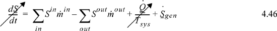
The left-hand side drops out because the system is at steady state. If the device is reversible, ![]() is zero. Further, these devices typically have a single inlet or outlet,17 and
is zero. Further, these devices typically have a single inlet or outlet,17 and ![]() , thus,
, thus,
Therefore, if we know the inlet state, we can find Sin. The outlet pressure is generally given, so for a pure fluid, the outlet state is completely specified by the two state variables Sout and Pout. We then use thermodynamic relations to find the other thermodynamic variables at this state, and use the energy balance at this state to find Wrev. Turbines, compressors, and pumps are very common equipment in chemical processes. Guidelines exist for estimating the degree of irreversibility in each piece of equipment based on experience. These guidelines take the form of an estimated efficiency. For example, a large expensive turbine might be 85% efficient, but a small cheap one might be 65% efficient. To apply these guidelines, we must formally define efficiency, then familiarize ourselves with variations on how to characterize the capacity and operating conditions of these operations.
4.7. Turbine, Compressor, and Pump Efficiency
Our analysis of the Carnot devices supports statement 2 at the beginning of Section 4.3. We have seen that work is maximized/minimized when the entropy generation is zero. Analysis of other processes would verify this useful conclusion. Work is lost by processes which generate entropy. If a device is not internally reversible, work will be lost within the device. Also, even if the device is internally reversible, work may be lost by irreversible interactions with the surroundings. Therefore, in setting up and solving problems to find maximum/minimum work, the objectives must be clear as to whether the system is internally reversible or whether the entire process is reversible. When we apply the entropy balance to a reversible process, the term representing entropy generation is zero.
In Chapter 2, both velocity gradients and friction were discussed as phenomena that lead to irreversibilities. Indeed, entropy is generated by both of these phenomena as well as by heat conduction along temperature gradients discussed in this chapter. Considering factors which affect reversibility (generation of entropy), you may have challenged yourself to consider a practical way to transfer heat with only infinitesimal temperature differences, or move fluid with only infinitesimal velocity gradients. You are probably convinced that such a process would not be practical. Indeed, the rate at which heat is transferred increases as the temperature driving forces increase, and we need finite temperature differences to transfer heat practically. Likewise, a pump will have large velocity gradients. Although we can measure changes in other properties by which we can calculate entropy changes arising from irreversibilities, an a priori prediction of lost work (Wlost) or entropy generated (Sgen) is extremely difficult and generally impractical. Direct evaluation of lost work in process equipment, such as turbines and compressors, is far beyond routine calculation and determined by empirical experience. It may seem that all of the effort to characterize reversible processes will be difficult to relate to real processes.
However, we can use practical experience to relate real processes to the idealized reversible processes. Therefore, in analyzing or designing processes involving operations of this nature, it is often necessary to approximate the real situation with a reversible one in which (Wlost) = 0 (no entropy generation). Past experience with many devices, such as compressors and turbines, often permits the engineer to relate performance under hypothetical reversible conditions to actual operation under real conditions. The relation is usually expressed by means of an efficiency factor. Equipment manufacturers typically provide performance curves as a function of process conditions. For introductory purposes, in this text we use a fixed factor. For devices such as pumps and compressors which utilize work from the surroundings, efficiency is defined as
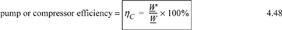
where the ′ denotes the reversible work. This notation will be used throughout the text when irreversible and reversible calculations are performed in the same problem. For turbines and other expansion devices that supply work to the surroundings, the definition is inverted to give
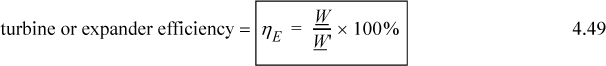
For adiabatic pumps, compressors, turbines, or expanders, the work terms may be calculated from the reversible and irreversible enthalpy changes by application of the energy balance.
Note: The strategy is to first calculate the work involved in a reversible process, then apply an efficiency which is empirically derived from previous experience with similar equipment. The outlet pressure of an irreversible adiabatic turbine or pump is always at the same pressure as a reversible device, but the enthalpy is always higher for the same inlet state. This means that if the outlet of the reversible adiabatic device is a single phase, the outlet of the irreversible adiabatic device will be at a higher temperature. If the outlet of the reversible adiabatic device is a two-phase mixture, the quality for the irreversible adiabatic device will be higher or the outlet could potentially be a single phase.
4.8. Visualizing Energy and Entropy Changes
Turbines, compressors, and pumps occur so frequently that we need convenient tools to aid in process calculations. Visualization of the state change is possible by plotting entropy on charts. This technique also permits the charts to be used directly in the process calculations. One common representation is the T-S chart shown in Fig. 4.6. The phase envelope appears as a fairly symmetrical hump. A reversible turbine, compressor, or pump creates state changes along a vertical line on these coordinates. Lines of constant enthalpy and pressure are also shown on these diagrams, as sketched in the figure. Volumes are also usually plotted, but they lie so close to the pressure lines that they are not illustrated in the figure here to ensure clarity.

Figure 4.6. Illustration of a T-S diagram showing lines of constant pressure and enthalpy.
![]() Visualizing state changes on charts will be helpful when using tables or computers for physical properties.
Visualizing state changes on charts will be helpful when using tables or computers for physical properties.
P-H diagrams shown in Fig. 4.7 are also useful; they are used frequently for refrigeration processes. The phase envelope tends to lean to the right because the enthalpies of vapor and liquid are both increasing along the saturation curve until the critical point is approached, where the vapor-phase enthalpy decreases due to significant non-idealities. Lines of constant entropy on these plots are slightly diagonal with a positive slope as shown in Fig. 4.7(a). For some hydrocarbons and halogenated compounds, the phase envelope can lean more sharply than the isentropic lines as shown in Fig. 4.7(b). A reversible compressor will operate along a line of constant entropy.
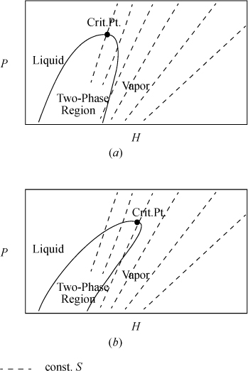
Figure 4.7. Illustration of a P-H diagram showing (a) lines of constant entropy for a species where the saturation curve leans less than isentropes (e.g., water) and (b) illustration of a P-H diagram showing lines of constant entropy for a species where the saturation curve leans more than isentropes (e.g., hexane).
Another convenient representation of entropy is the H-S diagram (Mollier diagram). In this diagram, lines of constant pressure are diagonal, and isotherms have a downward curvature as in Fig. 4.8. The saturation curve is quite skewed.
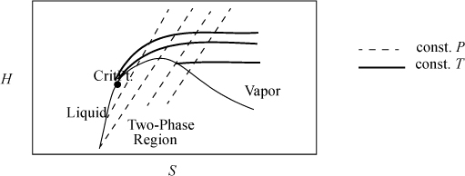
Figure 4.8. Illustration of an H-S (Mollier) diagram showing lines of constant entropy.
4.9. Turbine Calculations
For a reversible adiabatic turbine, the entropy balance in Section 4.6 shows that the outlet entropy must equal the inlet entropy. For an irreversible turbine, the outlet entropy must be greater than the inlet entropy. We may now visualize the state change on the diagrams sketched in Section 4.8. For example, on a T-S diagram, the performance of a turbine can be visualized as shown in Fig. 4.9. Note that the isobars are important in sketching the behavior because the outlet pressure must be the same for the reversible and irreversible turbines, but the outlet enthalpies (not shown) and entropies must be different.

Figure 4.9. Illustration of a reversible and actual (irreversible) turbine on a T-S diagram.
![]() The outlet entropy of an irreversible adiabatic turbine will be greater than the outlet entropy of a reversible adiabatic turbine with the same outlet pressure.
The outlet entropy of an irreversible adiabatic turbine will be greater than the outlet entropy of a reversible adiabatic turbine with the same outlet pressure.
Steam Quality Calculations
![]() The actual outlet state might be in the one-phase region when the reversible outlet state is in the two-phase region.
The actual outlet state might be in the one-phase region when the reversible outlet state is in the two-phase region.
A common problem encountered when adiabatically reducing the pressure of real fluids like steam, methane, or refrigerants is the formation of a vapor-liquid mixture. Since the thermodynamic properties change dramatically depending on the mass fraction that is vapor (the quality), it is important to know how to calculate that fraction. The calculation procedure may differ from the case shown in Fig. 4.9 where the outlets for the reversible and irreversible cases are both one phase. Since the reversible adiabatic turbine is isentropic, the line representing the reversible process must be vertical. As shown in Fig. 4.10, if the upstream entropy is less than the saturated vapor entropy at the outlet pressure, the reversible outlet ends up inside the liquid-vapor region, to the left of the saturated vapor curve. In this case, we must perform a quality calculation to determine the vapor fraction. Since the actual turbine must have an outlet state of higher entropy, due to entropy generation, the outlet state can lie inside the phase envelope, on the saturation curve, or outside the phase envelope, depending on the proximity of the reversible outlet state to the saturation curve and also depending on the turbine efficiency. A frequent question is, “How do I know when I need a quality calculation?” The calculation is required if the inlet entropy is less than the saturation entropy at the outlet pressure as illustrated in the figure. A quality calculation may also be required for the actual state, if the actual enthalpy turns out to be less than the saturation enthalpy at the outlet pressure.

Figure 4.10. Illustration of need for quality calculation on turbine outlet where the actual outlet is saturated steam.
The best way to master turbine calculations is to practice; the examples in this section are designed to facilitate your effort. Example 4.13 explores the inference of outlet conditions and proper application of turbine efficiency. Example 4.14 illustrates calculation of turbine efficiency. Example 4.15 illustrates the determination of inlet conditions to match a desired outlet. The combinations of inlet and outlet specifications are too many to enumerate. Therefore, you need to practice inferring the necessary procedure for any given situation. Challenge yourself to repeat the examples without looking at the steps. Several practice problems are also given at the end of the chapter, with detailed solutions available at the textbook web site. As you practice, pay attention to the results and look for generalities that broaden your comprehension.
Determining Turbine Outlet Conditions
Let us work a series of examples illustrating the various situations that may arise in calculation of turbine outlets. Usually, the design of a turbine involves a given inlet state and outlet pressure. That outlet pressure may be specified explicitly, or it may be implicit in a statement giving the outlet temperature and the quality; it may be inferred then that the outlet pressure is the saturation pressure at the given temperature. An important skill is to quickly determine whether the reversible turbine follows Fig. 4.9 or whether it follows Fig. 4.10. Subsequently, for the cases that follow Fig. 4.10, the outlet state may lie inside or outside the phase envelope. The determination depends on the efficiency and the inlet entropy, with the following cases:
i. Reversible outlet one phase, actual outlet one phase;
ii. Reversible outlet two phase, actual outlet one phase;
iii. Reversible outlet two phase, actual outlet two phase.
This example, though long, comprehensively covers the solution methods to determine turbine outlets for single-stage turbines from a known inlet state and specified pressure drop.
Example 4.13. Various cases of turbine outlet conditions
An adiabatic turbine inlet (state 1) is 500°C and 1.4 MPa. For each of the following outlet conditions (state 2), determine the specified quantities.
a. P2 = 0.6 MPa, ηE = 0.85. Find WS, H2, S2, and T2.
b. P2 = 0.03 MPa, ηE = 0.85. Find WS, H2, S2, and T2.
c. P2 = 0.01 MPa, ηE = 0.9. Find WS, H2, S2, and T2.
Note that using a common inlet state for each of the cases will permit us to skip the steps to determine the inlet state as we work the different alternatives.
Solution
First, the inlet properties are determined: H1 = 3474.8 kJ/kg, S1 = 7.6047 kJ/kg-K. The reversible calculation is performed for each outlet condition, recognizing that a reversible turbine is isentropic.
a. S2′ = S1 = 7.6047 kJ/kg-K. Comparing with SsatV= 6.7593 kJ/kg-K at P2 = 0.6 MPa, S2′ > SsatV, so the reversible outlet state is superheated and any irreversibility must lead to greater entropy and greater superheat (case (i)). This is the case of Fig. 4.9. Interpolating:
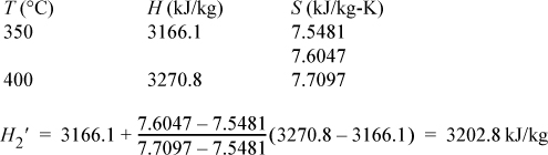
By similar interpolation, T2′ = 367.5°C.
ΔH′ = WS′ = 3202.8 – 3474.8 = –272.0 kJ/kg
Applying ηE calculation, ΔH = WS = ηEΔH′ = 0.85(–272) = –231.2 kJ/kg,
H2 = H1 + ΔH = 3474.8 – 231.2 = 3243.6 kJ/kg
Preparing for interpolation:

By similar interpolation, T2 = 387.0°C. We see that irreversibility has warmed the outlet, but not “heated” it, because it was adiabatic. With a one-phase outlet, T2 > T2′ if ηE < 1.
b. The pressure is lower than part (a), and the saturated vapor S will be larger, and near the saturation boundary.
Recall that S2′ = S1 = 7.6047 kJ/kg-K. Comparing with SsatV= 7.7675 kJ/kg-K at P2 = 0.03 MPa, S2′ < SsatV, so the reversible outlet state is two-phase. This is the case of Fig. 4.10 and we need to proceed further to determine if the actual state is inside or outside the phase envelope. Interpolating using the saturation entropy values along with the S2′ at T2′ = 69.1°C,
Using Eqn. 1.27:
H2′ = 289.27 + 0.976(2335.28) = 2568.5 kJ/kg
ΔH′ = WS′ = 2568.5 – 3474.8 = – 906.3 kJ/kg
Applying ηE calculation, ΔH = WS = ηE ΔH′ = 0.85(–906.3) = –770.35 kJ/kg,
H2 = H1 + ΔH = 3474.8 – 770.35 = 2704.4 kJ/kg
Comparing H2 with HsatV = 2624.55 kJ/kg at P2 = 0.03 MPa, H2 > HsatV, so the outlet state is superheated (outside the phase envelope). This is an instance of case (ii).
To conclude the calculations, a double interpolation is required. Performing the first interpolation between 0.01 and 0.05 MPa will bracket the outlet state. (Note: 0.03 MPa is halfway between 0.01 and 0.05 MPa, so tabulated values are obtained by averaging rather than by a slower interpolation.)
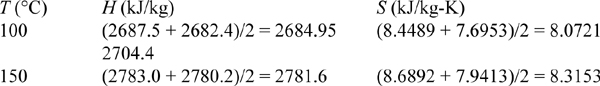
Interpolating:
Similarly, by interpolation, T2 = 110.1°C.
Note: The reversible state is two-phase, and the actual outlet is one-phase for part (b). Also, S2 > S2′ = S1 and H2 > H2′ which are always true for irreversible turbines. T2 > T2′, which is a general result for one-phase output.
c. Very low-outlet pressures shifts the saturation value of S to even higher values, making it more likely that the outlet will be two phase, case (iii).
S2′ = S1 = 7.6047 kJ/kg-K. Comparing with SsatV= 8.1488 kJ/kg-K at P2 = 0.01 MPa, S2′ < SsatV, so the reversible outlet state is two-phase. This is the case of Fig. 4.10 and we need to proceed further to determine if the actual state is inside or outside the phase envelope. Interpolating at P = 0.01 MPa (T2′ = 45.81°C),
Using Eqn. 1.27,
H2′ = 191.81 + 0.9274(2392.05) = 2410.2 kJ/kg
ΔH′ = WS′ = 2410.3 – 3474.8 = – 1064.6 kJ/kg
Applying ηE calculation, ΔH = WS = ηE ΔH′ = 0.90(–1064.6) = –958.1 kJ/kg,
H2 = H1 + ΔH = 3474.8 – 958.1 = 2516.7 kJ/kg.
Comparing H2 with HsatV = 2583.86 kJ/kg at P2 = 0.01 MPa, H2 < HsatV, so the actual outlet state is two-phase as well as the reversible outlet (case (iii)). For the actual outlet, H2 gives:
Using Eqn. 1.27,
S2 = 0.6492 + 0.972(7.4996) = 7.9388 kJ/kg
The actual outlet is wet steam at T2 = 45.81°C. The reversible outlet and the actual outlet are both wet steam for part (c). Also, S2 > S2′ = S1 and H2 > H2′ which are always true for irreversible turbines. For case (c), T2 = T2′, however q2 > q2′, a general result for a two-phase outlet.
This example has exhaustively covered the possibilities that may occur when performing turbine analysis given a specified pressure drop and known inlet condition. The actual outlet enthalpy and entropy are always greater than the reversible values. The actual outlet T will be the same as the reversible T if both states are wet steam. Note that many variations could generate calculations that appear to be different from these cases, but are actually similar. For example, the quality could be specified at the outlet instead of the efficiency. Similarly, the steam outlet H or S, etc. could be specified rather than the quality. For any problem, the details of the interpolation may differ for a given application depending on the region of the steam tables. Nevertheless, the overall procedures of using entropy to identify the reversible state and then correcting for the actual state are always the same. The following example illustrates a typical turbine calculation that might be used to characterize the efficiency of a working turbine.
Example 4.14. Turbine efficiency calculation
An adiabatic turbine inlet is at 500°C and 1.4 MPa. Its outlet is at 0.01MPa and q = 99%.
a. Compute the work of the turbine.
b. Compute the work of a reversible turbine.
c. Compute the efficiency of the turbine and the entropy generation of the actual turbine.
Solution
The energy balance is ΔH = WS.
a. The inlet is the same as Example 4.13: H1 = 3474.8; S1 = 7.6047. At the outlet,
H2 = 191.81 + 0.99(2392.05) = 2559.9 kJ/kg
ΔH = WS = 2559.9 – 3474.8 = –914.9 kJ/kg
b. Entropy balance: ΔS′ = 0 ⇒ S2′ = S1 = 7.6047 kJ/kg-K.
It is slightly ambiguous whether we should match the outlet pressure or the specification of quality. By convention, it is assumed that pressure is the desired criterion (or temperature in a similar situation) because this pertains to the physical constraints of the design. This means that the reversible work is the same as Example 4.13(c) and WS′ = –1064.6 kJ/kg.
c. The turbine efficiency is defined by ηE = WS/WS′ = 914.9/1064.6 = 85.9%. The entropy generation is given by Sgen = S2 – S2′.
S2 = 0.6492 + 0.99(7.4996) = 8.0738 kJ/kg-K
Referring to the entropy balance, S2′ = S1 = 7.3046 so Sgen = 8.0738 – 7.6047 = 0.4691 J/g-K.
Another type of calculation involves determining a turbine inlet that will result in a certain outlet. The procedure is to use the outlet state to estimate the inlet entropy as a crude guess, and then use trial and error inlet conditions until the desired outlet state is matched.
Example 4.15. Turbine inlet calculation given efficiency and outlet
An adiabatic turbine outlet (state 2) is 99% quality steam at 0.01 MPa, ηE = 85%. The inlet pressure has been specified as 0.6 MPa. An absolute pressure of 0.6 MPa is conventionally defined as low pressure steam and is often applied in chemical processing. Find WS, H1, S1, and T1.
Solution
“Coincidentally,” the outlet properties were determined in Example 4.14: H2 = 2559.9; S2 = 8.0738. Referring to the superheated steam tables at 0.6 MPa, we seek an entropy value that is less than 8.0738 kJ/kg-K because ηE < 100% means entropy is generated. This occurs around 500°C. Trying 500°C, gives H1 = 3483.4 kJ/kg and S1 = 8.0041 kJ/kg-K. Then WS = –923.5 kJ/kg; q′ = (8.0041 – 0.6492)/7.4996 = 0.9807;
So H1′ = 191.8 + 0.9807(2392)=2537.6 kJ/kg; WS′ = 2537.6 – 3483.4 = –945.8 kJ/kg;
Wlost = 945.8 – 923.5 = 22.3 kJ/kg; ηE = –923.5/(–923.5 – 22.3) = 97.7%.
Further trials generate the values tabulated below. The last temperature is estimated by interpolation. (Hint: It would be great practice for you to compute these and check your answers.).

Multistage Turbines
Commonly, turbines are staged for several reasons that we explore in Chapter 5. Generally, some steam is drawn off at intermediate pressures for other uses. The important point that needs to be stressed now is that the convention used for characterizing efficiency is important. Consider the three-stage turbine shown in Fig. 4.11 and the schematic that represents the overall reversible path and the actual path. The isobars on the H-S diagram for water curve slightly upward, and are spaced slightly closer together at the bottom of the diagram than at the top. The overall efficiency is given by ![]() , and the efficiency of an individual stage is given by
, and the efficiency of an individual stage is given by ![]() . If we consider the reversible work as ΔH′overall, that quantity must be smaller than
. If we consider the reversible work as ΔH′overall, that quantity must be smaller than ![]() . In fact, because the isobar spacing is increasing to the right of the diagram, the vertical drop between any isobars on the line marked as the overall reversible path must be smaller than the vertical drop between the same two isobars starting along the actual path (except for the very first turbine). Therefore, the efficiency calculated for the overall system must be higher than the efficiency for the individual stages. This comparison does not imply that staging turbines alters their performance. The difference in efficiencies is due to differences in what is considered to be the basis for the reversible calculation. The cautionary note to retain from this discussion is that the distinction between overall or individual efficiencies is important when communicating the performance of a staged turbine system.
. In fact, because the isobar spacing is increasing to the right of the diagram, the vertical drop between any isobars on the line marked as the overall reversible path must be smaller than the vertical drop between the same two isobars starting along the actual path (except for the very first turbine). Therefore, the efficiency calculated for the overall system must be higher than the efficiency for the individual stages. This comparison does not imply that staging turbines alters their performance. The difference in efficiencies is due to differences in what is considered to be the basis for the reversible calculation. The cautionary note to retain from this discussion is that the distinction between overall or individual efficiencies is important when communicating the performance of a staged turbine system.
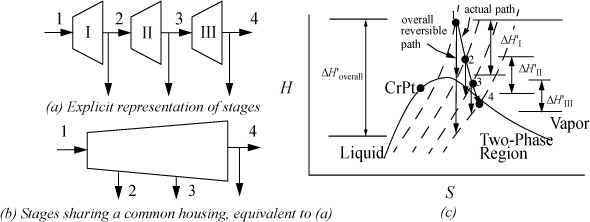
Figure 4.11. Illustration that overall efficiency of an adiabatic turbine will be higher than the efficiency of the individual stages.
4.10. Pumps and Compressors
An irreversible, adiabatic pump or compressor generates entropy. If these devices are reversible, they are isentropic. Examples of both are shown in Fig. 4.12. The calculations are generally straightforward. Consider the case where the inlet state and the outlet pressure is known. First, the reversible outlet state is determined based on the isentropic condition, and the enthalpy at the reversible state is known. The most common estimate for compressors is described in Example 2.12 on page 76. Even though it is intended for ideal gases, it is convenient for many applications and often provides a reasonable first approximation. The most common estimate for pumps is described in Eqn. 2.32 on page 55. These both pertain to reversible processes. The efficiency can then be used to determine the actual outlet enthalpy and work, using Eqn. 4.46.
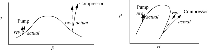
Figure 4.12. Illustrations of pathways for reversible and irreversible pumps and compressors. The P-H diagram is for a system like Fig. 4.7(a).
Example 4.16. Isothermal reversible compression of steam
In Example 2.12 on page 76, we mentioned that computing the work for isothermal compression of steam was different from computing the work for an ideal gas. Now that you know about the entropy balance, use it to compute the work of continuously, isothermally, and reversibly compressing steam from 5 bars and 224°C to 25 bars. Compare to the result of the ideal gas formula.
Energy balance: ΔH = Q + W. Entropy balance: ΔS = Q/T. Note that ΔS ≠ 0, even though this is a reversible process. Sgen = 0, but the process is not adiabatic. From the steam tables, we note that 224°C and 25 bars is practically equal to the saturated vapor. For the vapor at 224°C and 25 bars, interpolation gives H = 2910.5, S = 7.1709. Noting Q = TΔS, Q = (224 + 273.15)(6.2558 – 7.1709) = –454.94; W = (2801.9 – 2910.5) + 454.94 = 346.3 J/g.
By the ideal gas formula, W = 8.314(4.04)(224 + 273.15)ln(5)/18 = 1493.1 J/g.
The work is less for the real vapor because of the intermolecular attractions. The difference was particularly large in this case because the final pressure was fairly high (> 10 bars).
Multistage Compression
During adiabatic compression of vapors, the temperature rises. This can cause equipment problems if the temperature rise or pressure ratio (Pout/Pin) is too large. To address this problem, interstage cooling is used to lower the gas temperature between compression stages. Such operations are common when high pressures need to be reached. A schematic of a compressor with interstage cooling is shown in Fig. 4.13. The total work for multistage compression is generally given by summing the work of each stage using Eqn. 2.69 on page 77. However, the ideal gas law becomes less reliable as the stagewise inlet pressure increases. If the inlet pressure is above 10 bars and the reduced temperature is less than 1.5, nonideality effects should be evaluated. Methods to evaluate gas non-idealities and to calculate entropy for all manner of non-ideal gases are discussed in Unit II. For common refrigerants, it is convenient to apply charts that are functionally equivalent to the steam tables. The charts are difficult to read and precision is relatively low compared to using the steam tables. Example 4.17 illustrates the procedure using the refrigerant R134a.

Figure 4.13. Illustration of a multistage compression and the corresponding P-H diagram. On the P-H diagram, the compressors appear as the curves of increasing pressure and the heat exchangers are the horizontal lines at constant pressure.
Example 4.17. Compression of R134a using P-H chart
A compressor operates on R134a. The inlet to the compressor is saturated vapor at –20°C. The outlet of the compressor is at 7.7 bar and ηC = 0.8. Find the reversible and required work (kJ/kg) and the outlet temperature of the compressor.
An inset of the P-H diagram from Appendix E is shown below. The axis labels and superheated temperature labels have been translated on the inset diagram.
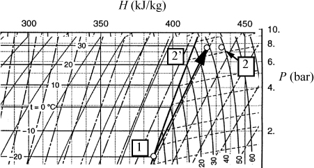
The inlet state is located at the intersection of the –20°C isotherm and the saturated vapor line. The enthalpy is found by following the vertical lines to the axis and H = 386.5 kJ/kg. (Note: This accurate value was found from the accompanying saturation table, but the schematic value is consistent, though less accurate.) The reversible outlet state is found by following an isentropic state up to 7.7 bars. One set of the diagonal lines are isentropes, and we visually interpolate to keep the same relative position between the isentropes at 7.7 bar at the state labeled 2′. By following the vertical lines to the axis, H2′ = 424 kJ/kg. The reversible work is WS′ = 424 – 386.5 = 37.5 kJ/kg. The actual work is WS = WS′ / 0.8 = 47 kJ/kg. The actual outlet state is shifted to the right at 7.7 bar at an enthalpy value of H2 = 386.5 + 47 = 433.5 kJ/kg. The reversible outlet is just near 38°C. The actual outlet is near 48°C.
4.11. Strategies for Applying the Entropy Balance
When solving thermodynamic problems, usually the best approach is to begin by applying the mass and energy balances. The entropy balance provides another balance, but it is not always necessary for every problem. In this chapter, we have introduced some new terms which can specify additional constraints when used in the problem statement, e.g., “isentropic,” “reversible,” “internally reversible,” “irreversible,” “thermal efficiency,” and “turbine/expander or compressor/pump efficiency.”
The entropy balance is useful to calculate maximum work available from a process or to evaluate reversibility. The entropy balance should be introduced with care because it is often redundant with the energy balance when simplified with information from step 5 from the strategies of Section 2.13. (For example, the entropy balance applied to Example 2.11 on page 75 results in the same simplified equation as the energy balance.) In general, if the pressures and temperatures of the process are already known, the entropies at each point, and the entropy changes, can be determined without direct use of the entropy balance. However, if either the pressure or the temperature is unknown for a process, the entropy balance may be the key to the solution.
![]() In some cases, T and P are known, so S can be determined without the entropy balance in a pure system.
In some cases, T and P are known, so S can be determined without the entropy balance in a pure system.
Before beginning more examples, it is also helpful to keep in mind those processes which generate entropy. This is important because, in the event that such processes arise, the entropy-generation term cannot be set to zero unless we modify the process to eliminate the source of the generation. Entropy is generated by the following processes.
1. Heat conduction along a temperature gradient.
2. Diffusion along a concentration gradient.
3. Mixing of substances of different composition.
4. Adiabatic mixing at constant system volume of identical substances initially at different molar entropies due to (T, P) differences.
5. Velocity gradients within equipment. This is accounted for in pipe flow by the friction factor developed in textbooks on fluid flow.
6. Friction.
7. Electrical resistance.
8. Chemical reactions proceeding at measurable rates.
In an open system, irreversibilities are always introduced when streams of different temperatures are mixed at constant pressure (item 4 above) because we could have obtained work by operating a heat engine between the two streams to make them isothermal before mixing. If the streams are isothermal, but of different composition, mixing will still generate entropy (e.g., see Eqn. 4.8 on page 138), and we have not yet devised a general method to obtain work from motion on this molecular scale.
![]() Problem statements will rarely explicitly point out entropy generation, so you will need to look for causes.
Problem statements will rarely explicitly point out entropy generation, so you will need to look for causes.
As chemical engineers, it is important to recognize that all chemical reactions proceeding at a finite rate generate entropy. The fundamental proof of this is provided in Section 17.16 and requires discussion of the chemical potential discussed much later in the text. Like the other processes listed here, reactions proceed spontaneously toward an equilibrium state due to finite driving forces. It is possible to calculate the rate of entropy generation if the chemical potentials are known at the reaction conditions. However, do not be deceived into thinking that a realistic reaction is thermodynamically reversible. Reaction engineering literature refers to reactions as reversible if the equilibrium constant (to be discussed later) is near 1 because the reaction can go “in either direction” (forward/backward) depending on the driving forces. This type of reversibility is not the same as thermodynamic reversibility. The reaction proceeding in either direction at measurable rates will generate entropy and be thermodynamically irreversible.
When a situation requires the minimum work input, or the maximum work output, the system is designed to minimize entropy generation, or make it zero if possible considering the limitations discussed here. As we work examples, recall the comments from Section 3.4 which we repeat here:
Note: For irreversible processes, note that we do not apply the entropy balance to find entropy changes. We always calculate the entropy change by an alternate reversible pathway that reaches the final state, then we apply the entropy balance to find how much entropy was generated, or we find the reversible work, apply an efficiency factor, and identify the final state via the energy balance.
Alternatively, for reversible processes, we do apply the entropy balance because we set the entropy generation term to zero.
4.12. Optimum Work and Heat Transfer
Let us consider how to calculate the optimum work interactions for a general system. For an open system where kinetic energy and potential energy changes are negligible,
where dSgen = 0 for an internally reversible process. If all the heat is transferred at a single temperature Tsys, elimination of dQ in the first balance provides

If we wish to apply this balance to a process that is conceptually reversible, we must use care to avoid any processes that are inherently irreversible (throttle valves, composition mixing processes, mixing of streams with identical composition but different temperatures, standard heat exchangers, chemical reactions at finite rates). Thus, if we consider a process that involves mixing compositions or reactions, we must include realistic estimates of these terms before determining the optimum work interaction. Once we recognize these limitations, we are ready to consider the general problem of finding optimum work interactions.
Availability (Exergy)
Section 4.5 considered optimum work interactions between a closed system and reservoir and found that optimum work interactions occur when the system temperature where heat transfer occurs is equal to the reservoir temperature. Therefore, for optimum work interactions with the surroundings, Tsys in Eqn. 4.52 should be replaced with the surrounding’s temperature To. Though it leads to optimum work, it is an idealized condition because the rate of heat transfer is proportional to the temperature difference (as studied in heat transfer courses), and the heat transfer with infinitesimal temperature differences will be infinitesimally slow. The surrounding’s temperature and pressure (To and Po) are often considered the dead state, because when the system reaches this T and P, energy input of some type is necessary to obtain expansion/contraction work, shaft work, or heat transfer; without energy input the process is dead. However, departures from this dead state do provide opportunities for work and heat interactions. Further, it is desirable to give a name to the combination of variables that results. For the combination of variables in the summations of Eqn. 4.52 modified with To, we will use the term availability, or exergy, B,
where H and S are state properties of the system at T and P, but To is the temperature of the dead state. The terms “availability” and “exergy” are both used in literature for this property. At a given T and P, the availability changes with To, so B is somewhat different from other state properties used to this point. Inserting the availability into Eqn. 4.52, and collecting the state changes of the system on the left-hand side, results in a general balance (ignoring kinetic and potential energy like before),
Steady-State Flow
For a system at steady-state flow, all terms on the left-hand side drop out, resulting in
and we conclude that the difference in availability from the inlets to outlets is related to the optimum shaft work. Note that TodSgen ≥ 0 and always subtracts from work input when dWS ≥ 0 which means work input for an irreversible process is always greater than a reversible process for a given state change. Similarly, for a given state change producing work, an irreversible process will always produce less work compared to a reversible process. The quantity ToSgen is called the lost work and the reason for the term should now be obvious. To is ambiguous when no heat is transferred to the surroundings and drops out for an adiabatic process such as an adiabatic turbine without any loss in applicability of the equation,
Closed System
For a closed system, Eqn. 4.54 becomes
Josiah Willard Gibbs (1839–1903) was an American chemist, mathematician, and physicist. Yale University awarded Gibbs the first American Ph.D. in Engineering in 1863 and Gibbs spent his career there. Gibbs is recognized for applying calculus to thermodynamics and combining the first and second laws. Gibbs studied the concept of chemical potential, the Gibbs phase rule, and many other relations.
For a constant-pressure closed system, VdP can be added to the left side (because it is zero in magnitude), which then results in dU + PdV + VdP = dU + d(PV) = dH. Thus, the left-hand side can be replaced with dB, though it is usually easier to calculate dH and TodS independently. We can define the Gibbs energy G ≡ H – TS. Then dG = dU + PdV + VdP – TdS – SdT. Thus, if the pressure is constant and the temperature is constant at To, then the change in Gibbs energy is related to the non-expansion/contraction work. Another interesting analysis can be done if both work terms are on the right-hand side of the equation:
Hermann Ludwig Ferdinand von Helmholtz (1821–1894) was a German physician and physicist.
Besides studying optics of the eye, he studied the concept of conservation of energy.
We can define the Helmholtz energy A ≡ U – TS. Then dA = dU – TdS – SdT. When the system is isothermal at To, then the change in Helmholtz energy is related to the sum of all forms of work.
Availability Analysis
As the world population grows and energy use increases, energy conservation will become increasingly important. Not only is the energy balance important, but so is the wise use of existing resources. Availability analysis can be used to determine how much entropy is generated by a process. Availability analysis is sometimes used in process design analysis,18 and may be used more widely in the future as we consider wise stewardship of energy resources.
Minimum Work for Separation
A key challenge in the development of a fermentation process is the titer, or yield from the fermentation. Fermentation is used in the pharmaceutical industry to develop natural molecules. For example, bacterial production of insulin is a feasible technology. Much of the cost of production depends on the dilution level. We can estimate the minimum energy cost for concentrating a product by combining the energy and entropy balances. Suppose that for a feed F we wish to obtain a pure product P and by-product water, B, in an isothermal process. For continuous separation of a mixed stream, the steady-state energy balance for a reversible separation is
Assuming an ideal solution, we can recognize that because the heat of mixing is zero the energy balance becomes
The energy balance thus simplifies to
The steady-state entropy balance for reversible separation exchanging heat at T is:
The strategy will be to determine the heat transfer from the entropy balance and then use it in the energy balance to find the work.
The entropy of the feed stream will be (using Eqn. 4.9)
Inserting,

which becomes
Let us suppose that component 2 is the desired species. On the basis of heat transfer per mole of component 2,

Combining with the energy balance, the minimum work per mole of desired species is
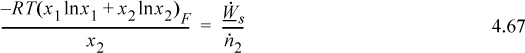
Example 4.18. Minimum heat and work of purificationa
Products produced by biological systems can range over mole fractions from 10–1 to 10–9.
a. Estimate the minimum reversible heat and work requirement to purify one mole of product at 298.15 K over this range.
b. To understand the concentrations in dilute mixtures, calculate the mole fraction of insulin in 0.1wt% aqueous solution.
Solution
The work is from Eqn. 4.67, and the heat will have the opposite sign.
For x2 = 0.10, x1 = 0.9. At 298.15K,
Repeating the calculation for other values of x2:.
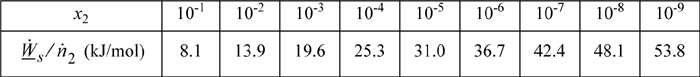
Note that heat must be rejected. If a process is envisioned that requires heat, then the rejected heat must be increased by an equal amount. For example, if a solution of concentration x2 = 0.10 is purified by adding 1 kJ of heat, then 9.1 kJ must be rejected.
(b) Searching for the molecular weight of insulin reveals a value of 5808 g/mol. Therefore, x1 = 0.001/5808 = 1.72(10-7). The point is that biomolecules are often large, and therefore their concentrations can be quite small on a mole fraction basis.
a. This problem was suggested by O’Connell, J.P. et al. July 2010. NSF BioEMB Workshop, San Jose, CA
4.13. The Irreversibility of Biological Life
A fascinating feature of living systems is that they organize small molecules into large structures. Towering pines grow with energy from the sun, CO2, water, and minerals extracted from the ground. Mammals grow into sophisticated thinking creatures by consuming small bits of food, consuming water, and breathing air. Small mindless flagella are known to swim “up” a concentration gradient toward a food source in a process known as chemotaxis. All of biological life builds molecules that are chiral rather than racemic. Don’t these processes violate the principles developed thus far in this chapter where we indicated the tendency of a system to move toward randomness? A careful analysis shows that the answer is no.
The key is that the feasibility of a process is determined by the entropy change of the universe, not the system itself. If organisms build molecules with lower entropy than the reactants, then the surroundings must increase in entropy by a larger amount. These changes can occur by control of the flux of molecules in/out of the system or by heat transfer. Mammals in particular are warmblooded, and are virtually isothermal. The body temperature of a healthy human being is universally 37°C (310 K). Rearrangement of the entropy balance for a human provides
Technically, if we assume T = 310K, we also should recognize that entropy is generated at the boundary between the human and the surroundings (at a lower temperature) and this is not included.
Every biochemical reaction in the body continuously generates entropy. If the organism is fully grown, we can approximate an adult as a steady-state process, so the first term on the left is nearly zero. The second term on the left contributes a negative value because entropy is generated constantly by the biochemical reactions. Ignoring transport terms initially, we can see that the heat transfer is expected to be negative. The magnitude depends on the entropy flows entering and leaving the system. Considering the other limiting possibility of negligible heat transfer, the entropy flow “in” must be less than the entropy flow “out.” In practice, these fluxes are not sufficient to sustain life. For humans, we know that our bodies reject heat at a rate of about 100 J/s. Thus, in addition to changing the entropy of our food to waste products, our existence depends on the ability to reject heat to the surroundings and thus contribute to increase the entropy of the surroundings via heat transfer. In the event that the surrounding temperature rises, humans experience heat stroke because the biological processes stop working when the heat transfer is not possible.
Trees and plants use photosynthesis to convert light energy (photons), to run the reaction
We have not explicitly included photons in our energy balance thus far, but it is a form of radiation similar to heat. A key point is that this reaction is not spontaneous as written. We discuss the driving forces for chemical reactions towards the end of the text, but a superficial discussion is relevant here. This reaction is an oversimplification of the actual process. In fact, more than 100 steps are needed for photosynthetic construction of glucose,19 but these steps drive the overall reaction above. To create a forward reaction, biological systems have developed a complex series of steps, each spontaneous and coupled such that carbohydrate production is possible. Plants are able to maintain this reaction by increasing the entropy of the surroundings to a greater extent than this reaction decreases the entropy when turning small molecules into carbohydrates.
Energy usage is inherently less efficient as we move up the food chain. When a herbivore or omnivore eats plant material, the stomach and intestinal enzymes break down the carbohydrates to simple sugars in catabolic reactions (a step that increases entropy). These sugars are then “burned” to produce CO2 (increasing entropy) as we showed in the previous chapter and the energy is used to maintain the life cycle and continuously produce new cells (anabolic reactions, decreasing entropy20) to replace dying cells and maintain tissue. Also, ingested proteins are broken into amino acids (increasing entropy) and then reassembled into new proteins (decreasing entropy2). As discussed above, only a portion of the energy provided by glucose can be utilized for biological maintenance; some must be rejected as heat. Each creature in the food chain repeats this “loss” of energy as heat is rejected. As engineers grapple with the challenge to use energy efficiently, it is helpful to keep in perspective that despite the complexity of living entities, the fundamentals of life are governed by the same principles as those developed in this chapter. Furthermore, life is made possible in humans by rejecting heat to the surroundings to drive the biological machinery. Despite their complexity, humans are not able to use all the energy generated by burning sugars.
4.14. Unsteady-State Open Systems
We end the chapter by providing examples of unsteady-state open systems. The first example shows that analysis of such systems can produce results quite consistent with expansion in a piston/cylinder.
Example 4.19. Entropy change in a leaky tank
Consider air (an ideal gas) leaking from a tank. How does the entropy of the gas in the tank change? Use this perspective to develop a relation between Tf and Pf and compare it to the expression we obtained previously by the energy balance.

m-Balance: dn = – dnout
S-Balance: ![]()
But physically, we know that the leaking fluid is at the same state as the fluid in the tank; therefore, the S-balance becomes ![]() , or ΔS = 0.
, or ΔS = 0.
For an ideal gas with a constant heat capacity:
Compare with Example 2.15 on page 81. The entropy balance and energy balance in this case are not independent. Either can be used to derive the same result. This also shows that our analysis in Example 2.15 was assumed to be reversible.
The next example builds on the first by adding a turbine to the tank. Note the method by which the system is subdivided to solve the problem.
Example 4.20. An ideal gas leaking through a turbine (unsteady state)
A portable power supply consists of a 28-liter bottle of compressed helium, charged to 13.8 MPa at 300 K, connected to a small turbine. During operation, the helium drives the turbine continuously until the pressure in the bottle drops to 0.69 MPa. The turbine exhausts at 0.1 MPa. Neglecting heat transfer, calculate the maximum possible work from the turbine. Assume helium to be an ideal gas with CP = 20.9 J/mol-K.

Consider a balance on the tank only. The result of the balance will match the result of Example 4.19.
Writing an entropy balance for a reversible adiabatic turbine only,
which shows that the turbine also does not change the molar entropy. Thus, the molar entropy of the exiting fluid is the same as the entropy in the tank, which is identical to the molar entropy at the start of the process. Therefore, the molar entropy and the pressure of the exiting gas are fixed. Since only two intensive properties fix all other intensive properties for a pure fluid, the exiting temperature is also fixed. The relation for an ideal gas along a reversible adiabat gives:
Solution by overall energy balance:
d(nU) = Hout dn + dWS and Hout is fixed since Tout, Pout are fixed; therefore, we may apply hint 4(a) from Section 2.14.
Integrating this expression:
nfUf – niUi = Hout(nf – ni) + WS
Rearranging:
Determining variables in the equation:
Choose reference temperature, TR ≡ 300 K, ⇒ setting UR = 0, then since HR = UR + (PV)R, and since the fluid is an ideal gas, CV = CP – R = 20.9 – 8.314 = 12.586 J/mol-K:
Now, plugging into Eqn. 4.70:
WS = 25.5(–2629 + 2892) – 154.9(0 + 2892)
⇒ WS = –441,200 J
4.15. The Entropy Balance in Brief
In this section, we refer to a division of the universe into the same three subsystems described in Section 2.14 on page 74.
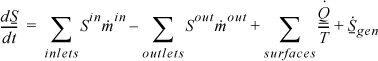
1. T is the system temperature at the location where Q is transferred.
2. Sin, Sout are state variables, and any pathway may be used to calculate the change from inlet to outlet. The pathway for calculation does not need to be the pathway for the actual process.
3. ![]() represents entropy generation due to irreversibilities within the system, e.g., internal heat transfer or conduction, viscous dissipation or mixing of streams of differing composition, or degradation of mechanical energy to thermal energy. Entropy generation at system boundaries is not included in the balance.
represents entropy generation due to irreversibilities within the system, e.g., internal heat transfer or conduction, viscous dissipation or mixing of streams of differing composition, or degradation of mechanical energy to thermal energy. Entropy generation at system boundaries is not included in the balance.
4. Entropy generation may occur at container walls. The entropy generation of the universe must be calculated by summing ![]() for all three subsystems, not just system 1 and system 3.
for all three subsystems, not just system 1 and system 3.
Test Yourself
1. What are the constraints on the sign of ![]() ?
?
2. Consider two isothermal processes both rejecting heat at the same temperature. One process is reversible and the other is irreversible. Which has a larger absolute value of heat transfer?
4.16. Summary
We began the chapter introducing microscopic methods to calculate entropy. We demonstrated that entropy increases when volume (for a gas) or temperature increases. Thermal energy is really a means of representing the randomness due to accessible microstates, such that the concept is best understood in terms of the microscopic definition of entropy. We showed that the macroscopic definition was consistent with the microscopic definition. We showed that entropy is essential for analysis of reversibility for processes, because irreversible processes generate entropy. We demonstrated that reversible Carnot cycle thermal efficiency was easily evaluated using entropy. The primary impact for pure-fluid applications is that compressors and turbines can be analyzed using empirical efficiencies relative to reversible devices. On a broader scale, however, you should appreciate the limitations of the conversion of heat into work.
This chapter is relatively long because mastering computations involving entropy can be challenging. Students may be familiar with energy balances and heats of reaction from previous courses, but entropy may seem new and abstract. Therefore, many examples have been provided. Students are encouraged to review these and the practice problems at the end of the chapter. The best way to develop a comfort level with entropy is to practice and learn by doing.
Important Equations
Entropy is a state change, and for an ideal gas,
For a condensed phase, the first term of the second equation should be used for a first approximation using the heat capacity for the appropriate phase.
Of course, the most important equation of this chapter is the complete entropy balance, but it may be convenient to remember some of its most common simplifications.
ΔS = 0 for a fluid in an adiabatic reversible process, like across a steady-state adiabatic reversible compressor or turbine or within an unsteady-state adiabatic reversible piston/cylinder.
ΔS = Qrev/T for a fluid in any process, like an isothermal reversible compressor. For an irreversible process, we design a reversible pathway to the actual final state.
ΔS = 0 for a the entropy in a reversible adiabatic leaking tank.
Pay careful attention to the subtle distinctions between these equations. A common mistake is to write ΔS = 0 whenever you see the word “reversible.” Remember that reversibility is coupled to entropy generation, not directly to S or ΔS. For entropy changes of a fluid, a smart approach is to write ΔS = Qrev/T always and then scratch a line through Qrev after you deliberately determine that the process is adiabatic and reversible. A fluid in an irreversible adiabatic process will have an entropy change (and Qrev) even though the actual heat transfer is zero. Note that the entropy balance uses the actual heat transfer, Q, not Qrev. Only for a reversible process are they identical.
The distinction between ΔS = 0 and ΔS = 0 is perhaps subtler. By writing ΔS = 0, we emphasize that only the specific entropy of the fluid remains constant. When ΔS = 0 for an open system, the quantity ΔS = nfSf – niSi = SΔn will be non-zero whenever S is not at the reference state.
Disorder must increase if two different gases are mixed slowly and adiabatically, but it is difficult to see how to compute the entropy change from the macroscopic definition of dS. For ideal solutions, the relation developed from the microscopic approach is:
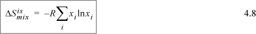
This equation is useful for estimating the effects of mixing in many situations, even beyond the assumption of ideal gases from which it derives. Eqn. 4.8 also conveys how disorder and mixing are not strictly related to heating, as one might infer from the macroscopic definition of entropy. The entropy of mixing will be of major importance in Unit III in the discussion of mixtures.
4.17. Practice Problems
P4.1. Call placement of a particle in box A, “heads” and placement in box B, “tails.” Given one particle, there are two ways of arranging it, H or T. For two particles, there are four ways of arranging them, {HH,HT,TH,TT}. We can treat the microstates by considering each particle in order. For example, {H T H H} means the first particle is in box A, the second in box B, the third in box A, and the fourth in box A.
a. List and count the ways of arranging three particles. Now consider four particles. What is the general formula for the number of arrangements versus the number of particles? (ANS. 2N)
b. How many arrangements correspond to having two particles in box A and one in box B? What is the probability of {2H,1T}? (ANS. 3/8)
c. How many arrangements correspond to {2H,2T}. {3H,2T}. {4H,2T}. {3H,3T}? (ANS. N!/[(N – m)!m!])
d. List the macrostates and corresponding number of microstates for an eight-particle, two-box system. What portion of all microstates are parts of either 5:3, 4:4, or 3:5 macrostates? (ANS. 71%)
e. What is the change of entropy in going from a 5:3 macrostate to a 4:4 macrostate? (ANS. 3.08E-24 J/K)
f. Use Stirling’s approximation to estimate the change of entropy in going from a distribution of 50.1% of 6.022E23 in box A to a distribution of 50.001%, and from 50.001% to 50.000%. (ANS. 1.2E18 J/K)
P4.2. Twenty molecules are contained in a piston + cylinder at low pressure. The piston moves such that the volume is expanded by a factor of 4 with no work produced of any kind. Compute ΔS/k. (ANS. 23.19)
P4.3. Fifteen molecules are distributed as 9:4:2 between equal-sized boxes A:B:C, respectively. The partitions between the boxes are removed, and the molecules distribute themselves evenly between the boxes. Compute ΔS/k. (ANS. 11.23)
P4.4. Rolling two die (six-sided cubes with numbers between 1 and 6 on each side) is like putting two particles in six boxes. Compute ΔS/k for going from double sixes to a four and three. (ANS. 0.693)
P4.5. Estimate the change in entropy when one mole of nitrogen is compressed by a piston in a cylinder from 300 K and 23 liters/mol to 400 K and 460 liters/mol. (CP = 7/2R) (ANS. 1.07 kJ/kgK)
P4.6. Steam at 400°C and 10 bar is left in an insulated 10 m3 cylinder. The cylinder has a small leak, however. Compute the conditions of the steam after the pressure has dropped to 1 bar. What is the change in the specific entropy of the steam in the cylinder? Is this a reversible process? The mass of the cylinder is 600 kg, and its heat capacity is 0.1 cal/g-K. Solve the problem with and without considering the heat capacity of the cylinder. (ANS. (a)~120°C; (b) 360°C)
P4.7. A mixture of 1CO:2H2 is adiabatically and continuously compressed from 5 atm and 100°F to 100 atm and 1100°F. Hint: For this mixture, CP = x1CP1 + x2CP2.
a. Estimate the work of compressing 1 ton/h of the gas. (CP = 7/2R) (ANS. 1.3E6 BTU/h)
b. Determine the efficiency of the compressor. (ANS. 76%)
P4.8. An adiabatic compressor is used to continuously compress nitrogen (CP/R = 7/2) from 2 bar and 300 K to 15 bar. The compressed nitrogen is found to have an outlet temperature of 625 K. How much work is required (kJ/kg)? What is the efficiency of the compressor? (ANS. 9.46 kJ/mol, 72%)
P4.9. An adiabatic compressor is used to continuously compress low-pressure steam from 0.8 MPa and 200°C to 4.0 MPa and 500°C in a steady-state process. What is the work required per kg of steam through this compressor? Compute the efficiency of the compressor. (ANS. 606 J/g, 67%)
P4.10. An adiabatic turbine is supplied with steam at 2.0 MPa and 600°C and the steam exhausts at 98% quality and 24°C. Compute the work output per kg of steam. Compute the efficiency of the turbine. (ANS. 1.2E3 kJ, 85%)
P4.11. An adiabatic compressor has been designed to continuously compress 1 kg/s of saturated vapor steam from 1 bar to 100 bar and 1100°C. Estimate the power requirement of this compressor in horsepower. Determine the efficiency of the compressor. (ANS. 3000 hp, 60%)
P4.12. Ethylene gas is to be continuously compressed from an initial state of 1 bar and 20°C to a final pressure of 18 bar in an adiabatic compressor. If compression is 70% efficient compared with an isentropic process, what will be the work requirement and what will be the final temperature of the ethylene? Assume the ethylene behaves as an ideal gas with CP = 44 J/mol-K. (ANS. 13.4 kJ/mol, 596 K)
P4.13. Operating a wind tunnel for aircraft experiments begins with adiabatically and reversibly compressing atmospheric air (300 K) into long cylinders comprising a total volume of 20 m3 at 200 bars. The cylinders are initially at 1 bar. Estimate the minimal amount of work required (MJ) to perform the compression step. (ANS. online.)
a. Write the most appropriate energy balance(s) for this process. Clearly identify the system(s) pertaining to your energy balance(s). Explain your reasoning briefly.
b. Write the most appropriate entropy balance(s) for this process. Clearly identify the system(s) pertaining to your entropy balance(s). Explain your reasoning briefly.
c. Solve for the minimal amount of work required (MJ) to perform the compression step.
P4.14. As part of a refrigeration cycle, Freon 134a is adiabatically compressed from the saturated vapor at –60°C (note the negative sign on temperature) to 1017 kPa and 100°C.
a. How much work is required in kJ/kg?
b. Estimate the efficiency of the compressor.
(ANS. 121, 75%)
P4.15. Steam is produced at 30 bar and some unknown temperature. A small amount of steam is bled off and goes through an adiabatic throttling valve to 1 bar. The temperature of the steam exiting the throttling valve is 110°C. What is the value of the specific entropy of the steam before entering the throttle? (ANS. 5.9736 J/g-K)
P4.16. Suppose the expansion in problem P2.19 was completely adiabatic instead of isothermal and CP = 7 cal/(mol-K). How would the height of the piston be affected? Must we generate heat or consume heat to maintain isothermal operation? (ANS. decrease, generate)
P4.17. It is desired to determine the volume of an initially evacuated tank by filling it from an 80 liter cylinder of air at 300 bar and 300 K. The final pressure of both tanks is 5 bars. Estimate the volume in liters. (ANS. 4720 L)
P4.18. An insulated cylinder is fitted with a freely floating piston, and contains 0.5 kg of steam at 9 bar and 90% quality. The space above the piston, initially 0.05m3, contains air at 300 K to maintain the pressure on the steam. Additional air is forced into the upper chamber, forcing the piston down and increasing the steam pressure until the steam has 100% quality. The final steam pressure is 30 bars, and the work done on the steam is 360 kJ, but the air above the steam has not had time to exchange heat with the piston, cylinder, or surroundings. The air supply line is at 50 bar and 300 K. What is the final temperature of the air in the upper chamber? (ANS. online)
P4.19. A well-insulated cylinder, fitted with a frictionless piston, initially contained 9 kg of liquid water and 0.4 kg of water vapor at a pressure of 1.4 MPa. 2 kg of steam at 1.6 MPa was admitted to the cylinder while the pressure was held constant by allowing the piston to expand. (ANS. online)
a. Write the energy balance for this process.
b. If the final volume of the contents of the cylinder was six times the initial volume, determine the temperature of the superheated steam that was admitted to the cylinder.
P4.20. Many action movies show gas cylinders that have their caps knocked off. The tanks go flying around wreaking havoc (only on the bad guys, of course). How much velocity could a tank like that really generate? For an upper bound, consider a tank traveling horizontally on a frictionless surface with an isentropic nozzle taking the place of the cap that has been knocked off. Suppose the cylinder weighs 70 kg and holds 50 L of He at 100bar, 300 K.
a. Write the most appropriate energy balance(s) for this process. Clearly identify the system(s) pertaining to your energy balance(s). Explain your reasoning briefly.
b. Write the most appropriate entropy balance(s) for this process. Clearly identify the system(s) pertaining to your entropy balance(s). Explain your reasoning briefly.
c. Solve for the total kinetic energy (MJ) developed by the tank and its velocity.
4.18. Homework Problems
4.1. Extending Example 4.2 on page 141 from solids to gases is straightforward if you recall the development of Eqn. 1.13 on page 19. Consider N2 for example. Being diatomic, we should expect that Uig = 2(3NAkT/2) = 6RT/2 in the limit of classical vibrations. Vibrational energy means that heat can be absorbed in the vibration of a bond. Since N2 has only one bond, it can only absorb energy in one way, removing one degree of freedom. We show in Eqn. 6.49 on page 240 that the change in energy due to vibration is ΔUvib = ε/[exp(—β ε) — 1]. For now, without concern for the proof, assume ΔUvib as given. Adapting Example 4.2 for N2 then gives: Uig = 5RT/2 + ε/[exp(—β ε) — 1].
a. Use the NIST WebBook to plot data for CV of N2 at 0.1 MPa and T = [150, 2000 K].
b. Derive an expression for CV based on above dissussion. Evaluate your expression at 1000K assuming ε/k = 1000K.
c. Regress an optimal value for ε/k of N2 and plot a comparison of the calculated results to experimental data. Show the calculated results as a curve with no points.
4.2. An ideal gas, with temperature-independent CP = (7/2)R, at 15°C and having an initial volume of 60 m3, is heated at constant pressure (P = 0.1013 MPa) to 30°C by transfer of heat from a reservoir at 50°C. Calculate ΔSgas, ΔSheat reservoir, ΔSuniverse. What is the irreversible feature of this process?
4.3. Steam undergoes a state change from 450°C and 3.5 MPa to 150°C and 0.3 MPa. Determine ΔH and ΔS using the following:
a. Steam table data
b. Ideal gas assumptions (be sure to use the ideal gas heat capacity for water)
4.4. The following problems involve one mole of an ideal monatomic gas, CP = 5R/2, in a variable volume piston/cylinder with a stirring paddle, an electric heater, and a cooling coil through which refrigerant can flow (see figure). The piston is perfectly insulated. The piston contains 1 gmole of gas. Unless specified, the initial conditions are: Ti = 25°C, Pi = 5 bar.
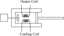
a. Status: Heater on; cooler off; paddle off; piston fixed. Five kJ are added by the heater. Find ΔU, ΔS, ΔP, and ΔT.
b. Status: Heater off; cooler off; paddle off; piston moveable. What reversible volume change will give the same temperature rise as in part (a)? Also find ΔU, ΔS, and ΔP.
c. Status: Heater off; cooler off; paddle on; piston fixed. What shaft work will give the same ΔU, ΔS as part (a)?
d. Status: Heater off; cooler off; paddle on; piston fixed. The stirring motor is consuming 55 watts and is 70% efficient. What rate is the temperature changing? At what initial rates are U and S changing?
e. Status: Heater unknown; cooler unknown; paddle off; piston free. We wish to perform a reversible isothermal compression until the volume is half of the initial volume. If the volume is decreasing at 2.0 cm3/s, at what rate should we heat or cool? Express your answer in terms of the instantaneous volume. What is the total heat transfer necessary?
4.5. When a compressed gas storage tank fails, the resultant explosion occurs so rapidly that the gas cloud can be considered adiabatic and assumed to not mix appreciably with the surrounding atmosphere. Consider the failure of a 2.5-m3 air storage tank initially at 15 bar. Atmospheric pressure is 1 bar, CP = 7R/2. Provide an estimate by assuming reversibility.
a. Calculate the work done on the atmosphere. Does the reversibility approximation overestimate or under-estimate the actual work?
b. A detonation of 1 kg of TNT releases about 4.5 MJ of work. Calculate the equivalent mass of TNT that performs the same work as in part (a).
4.6. Work problem 4.5 but consider a steam boiler that fails. The boiler is 250 L in size, operating at 4 MPa, and half full of liquid.
4.7. An isolated chamber with rigid walls is divided into two equal compartments, one containing gas at 600 K and 1 MPa and the other evacuated. The partition between the two compartments ruptures. Compute the final T, P, and ΔS for the following:
a. An ideal gas with CP/R = 7/2
b. Steam.
4.8. An isolated chamber is divided into two equal compartments, one containing gas and the other evacuated. The partition between the two compartments ruptures. At the end of the process, the temperature and pressure are uniform throughout the chamber.
a. If the filled compartment initially contains an ideal gas at 25 MPa and 650 K, what is the final temperature and pressure in the chamber? What is ΔS for the process? Assume a constant heat capacity of CP/R = 4.041.
b. If the filled chamber initially contains steam at 25 MPa and 650 K, what is the final temperature and pressure in the chamber? What is ΔS for the process? (Use the steam tables.)
4.9. Airplanes are launched from aircraft carriers by means of a steam catapult. The catapult is a well-insulated cylinder that contains steam, and is fitted with a frictionless piston. The piston is connected to the airplane by a cable. As the steam expands, the movement of the piston causes movement of the plane. A catapult design calls for 270 kg of steam at 15 MPa and 450°C to be expanded to 0.4 MPa. How much work can this catapult generate during a single stroke? Compare this to the energy required to accelerate a 30,000 kg aircraft from rest to 350 km per hour.
4.10. We have considered heat and work to be path-dependent. However, if all heat transfer with surroundings is performed using a reversible heat transfer device (some type of reversible Carnot-type device), work can be performed by the heat transfer device during heat transfer to the surroundings. The net heat transferred to the surroundings and the net work done will be independent of the path. Demonstrate this by calculating the work and heat interactions for the system, the heat transfer device, and the sum for each of the following paths where the surroundings are at Tsurr = 273 K. The state change is from state 1, P1 = 0.1 MPa, T1 = 298 K and state 2, P2 = 0.5 MPa and T2 which will be found in part (a). CP = 7R/2.
a. Consider a state change for an ideal gas in a piston/cylinder. Find T2 by an adiabatic reversible path. Find the heat and work such that no entropy is generated in the universe. This is path a. Sketch path a qualitatively on a P-V diagram.
b. Now consider a path consisting of step b, an isothermal step at T1, and step c, an isobaric step at P2. Sketch and label the step on the same P-V diagram created in (a). To avoid generation of entropy in the universe, use heat engines/pumps to transfer heat during the steps. Calculate the WEC and WS as well as the heat transfer with the surroundings for each of the steps and overall. Compare to part (a) the total heat and work interactions with the surroundings.
c. Now consider a path consisting of step d, an isobaric step at P1, and step e, an isothermal step at T2. Calculate the WEC and WS as well as the heat transfer with the surroundings for each of the steps and overall. Compare to part (a) using this pathway and provide the same documentation as in (b).
4.11. Consider the wintertime heating of a house with a furnace compared to addition of Carnot heat engines/pumps. To compensate for heat losses to the surroundings, the house is maintained at a constant temperature Thouse by a constant rate of heat transfer, ![]() . The furnace operates at a constant temperature TF, and with direct heat transfer, the heat required from the furnace,
. The furnace operates at a constant temperature TF, and with direct heat transfer, the heat required from the furnace, ![]() is equal to
is equal to ![]() .
.
a. Instead of direct heat transfer, if we utilize the surroundings, at TS, as an additional heat source and include heat pump technology, ![]() may be reduced by generating work from a heat engine operating between TF and TS, then applying that work energy to a heat pump operating between TS and Thouse. Given that TF = 800 K, T = 293 K, TS = 265 K, and
may be reduced by generating work from a heat engine operating between TF and TS, then applying that work energy to a heat pump operating between TS and Thouse. Given that TF = 800 K, T = 293 K, TS = 265 K, and ![]() = 40 kJ/h, determine
= 40 kJ/h, determine ![]() utilizing heat pump technology. No other sources of energy may be used.
utilizing heat pump technology. No other sources of energy may be used.
b. Another option is to run a heat engine between TF and Thouse and the heat pump between TS and Thouse. Compare this method with part (a).
4.12. An ideal gas enters a valve at 500 K and 3 MPa at a steady-state rate of 3 mol/min. It is throttled to 0.5 MPa. What is the rate of entropy generation? Is the process irreversible?
4.13. SO2 vapor enters a heat exchanger at 100°C and at a flowrate of 45 mole/h. If heat is transferred to the SO2 at a rate of 1,300 kJ/h, what is the rate of entropy transport in the gas at the outlet relative to the inlet in kJ/K/h given by ![]() ?
?
4.14. An ideal gas stream (Stream A), CP = 5R/2, 50 mole/h, is heated by a steady-state heat exchanger from 20°C to 100°C by another stream (Stream B) of another ideal gas, CP = 7R/2, 45 mole/h, which enters at 180°C. Heat losses from the exchanger are negligible.
a. For concurrent flow in the heat exchanger, calculate the molar entropy changes (Sout – Sin) for each stream, and ![]() for the heat exchanger.
for the heat exchanger.
b. For countercurrent flow in the heat exchanger, calculate the molar entropy changes (Sout – Sin) for each stream, and ![]() for the heat exchanger. Comment on the comparison of results from parts (a) and (b).
for the heat exchanger. Comment on the comparison of results from parts (a) and (b).
4.15. An inventor has applied for a patent on a device that is claimed to utilize 1 mole/min of air (assumed to be an ideal gas) with temperature independent CP = (7/2)R which enters at 500 K and 2 bar, and leaves at 350 K and 1 bar. The process is claimed to produce 2000 J/min of work and to require an undisclosed amount of heat transfer with a heat reservoir at 300 K. Should the inventor be issued a patent on this device?
4.16. Two streams of air are mixed in a steady-state process shown below. Assume air is an ideal gas with a constant heat capacity CP = 7R/2.
a. What is the temperature of the stream leaving the tank if the process is adiabatic?
b. What is the rate of entropy generation within the tank if the process is adiabatic?
c. If we duplicated the stream conditions (temperatures, pressures, and flowrates) with an internally reversible process, what is the maximum rate at which work could be obtained? If desirable, you are permitted to transfer heat to the surroundings at the surroundings’ temperature of 295 K.
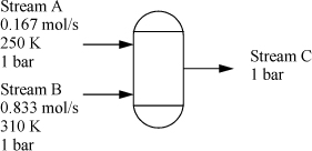
4.17. Air is flowing at steady state through a 5 cm diameter pipe at a flow rate of 0.35 mole/min at P = 5 bar and T = 500 K. It flows through a throttle valve and exits at 1 bar. Assume air is an ideal gas with CP = 29.1 J/mol-K. If the throttle valve was replaced by a reversible steady-state flow device to permit exactly the same state change for the air in this steady-state process, at what rate could work could be obtained? Heat transfer, if desired, can occur with the surroundings at 298 K, which may be considered a reservoir.
4.18. A common problem in the design of chemical processes is the steady-state compression of gases from a low pressure P1 to a much higher pressure P2. We can gain some insight about optimal design of this process by considering adiabatic reversible compression of ideal gases with stage-wise intercooling. If the compression is to be done in two stages, first compressing the gas from P1 to P*, then cooling the gas at constant pressure down to the compressor inlet temperature T1, and then compressing the gas to P2, what should the value of the intermediate pressure be to accomplish the compression with minimum work?
4.19. Steam flowing at steady state enters a turbine at 400°C and 7 MPa. The exit is at 0.275 MPa. The turbine is 85% efficient. What is the quality of the exiting stream? How much work is generated per kg of steam?
4.20. An adiabatic steam turbine inlet is to be 4 MPa. The outlet of the turbine is to operate at 0.01 MPa, and provide saturated steam. The turbine has an efficiency of 85%. Determine the superheat which is required on the turbine inlet, and the work produced by the turbine.
4.21. Steam is fed to an adiabatic turbine at 4 MPa and 500°C. It exits at 0.1 MPa.
a. If the turbine is reversible, how much work is produced per kg of steam?
b. If the turbine is 80% efficient, how much work is produced per kg of steam?
4.22. Methane is compressed in a steady-state adiabatic compressor (87% efficient) to 0.4 MPa. What is the required work per mole of methane in kJ? If the flow is to be 17.5 kmol/h, how much work must be furnished by the compressor (in kW)? What is the rate of entropy generation (in kJ/K/h)? (a) the inlet is at 0.1013 MPa and –240°F; (b) the inlet is 0.1013 MPa and 200 K.
4.23. Methane is to be compressed from 0.05 MPa and –120°F to 5 MPa in a two-stage compressor. In between adiabatic, reversible stages, a heat exchanger returns the temperature to –120°F. The intermediate pressure is 1.5 MPa.
a. What is the work required (kJ/kg) in the first compressor of methane?
b. What is the temperature at the exit of the first compressor (°C)?
c. What is the cooling requirement (kJ/kg) in the interstage cooler?
4.24. A steady stream (1000 kg/hr) of air flows through a compressor, entering at (300 K, 0.1 MPa) and leaving at (425 K, 1 MPa). The compressor has a cooling jacket where water flows at 1500 kg/hr and undergoes a 20 K temperature rise. Assuming air is an ideal gas, calculate the work furnished by the compressor, and also determine the minimum work required for the same state change of air.
4.25. Propane is to be compressed from 0.4 MPa and 360 K to 4 MPa using a two-stage compressor. An interstage cooler returns the temperature of the propane to 360 K before it enters the second compressor. The intermediate pressure is 1.2 MPa. Both adiabatic compressors have a compressor efficiency of 80%.
a. What is the work required in the first compressor per kg of propane?
b. What is the temperature at the exit of the first compressor?
c. What is the cooling requirement in the interstage cooler per kg of propane?
a. A steam turbine in a small electric power plant is designed to accept 5000 kg/h of steam at 60 bar and 500°C and exhaust the steam at 1 bar. Assuming that the turbine is adiabatic and reversible, compute the exit temperature of the steam and the power generated by the turbine.
b. If the turbine in part (a) is adiabatic but only 80% efficient, what would be the exit temperature of the steam? At what rate would entropy be generated within the turbine?
c. One simple way to reduce the power output of the turbine in part (a) (100% efficient) is by adjusting a throttling valve that reduces the turbine inlet steam pressure to 30 bar. Compute the steam temperature to the turbine, the rate of entropy generation, and the power output of the turbine for this case. Is this a thermodynamically efficient way of reducing the power output? Can you think of a better way?
4.27. Steam is used in the following adiabatic turbine system to generate electricity; 15% of the mass flow from the first turbine is diverted for other use.
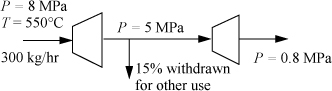
a. How much work (in kJ/h) is generated by the first turbine which is 80% efficient?
b. How much work (in kJ/h) is generated by the second turbine which is 80% efficient?
c. Steam for the turbines is generated by a boiler. How much heat must be supplied to the boiler (not shown) which has 300 kg/h of flow? The stream entering the boiler is T = 170°C, P = 8 MPa. The stream exiting the boiler matches the inlet to the first turbine.
4.28. Liquid nitrogen is useful for medical purposes and for research laboratories. Determine the minimum shaft work needed to liquefy nitrogen initially at 298 K and 0.1013 MPa and ending with saturated liquid at the normal boiling point, 77.4 K and 0.1013 MPa. The heat of vaporization at the normal boiling point is 5.577 kJ/mol, and the surroundings are at 298 K. The constant pressure heat capacity of gaseous nitrogen can be assumed to be independent of temperature at 7/2R for the purpose of this calculation.
a. Consider nitrogen entering a flow device at 1 mol/min. Give shaft work in kW.
b. Consider nitrogen in a piston/cylinder device. Give the work in kJ per mole liquefied.
c. Compare the minimum shaft work for the two processes. Is one of the processes more advantageous than the other on a molar basis?
4.29. Propane flows into a steady-state process at 0.2 MPa and 280 K. The final product is to be saturated liquid propane at 300 K. Liquid propane is to be produced at 1000 kg/h. The surroundings are at 295 K. Using a propane property chart, determine the rate of heat transfer and minimum work requirement if the process is to operate reversibly.
4.30. Propane (1000 kg/hr) is to be liquefied following a two-stage compression. The inlet gas is to be at 300 K and 0.1 MPa. The outlet of the adiabatic compressor I is 0.65 MPa, and the propane enters the interstage cooler where it exits at 320 K, then adiabatic compressor II raises the propane pressure to 4.5 MPa. The final cooler lowers the temperature to 320 K before it is throttled adiabatically to 0.1 MPa. The adiabatic compressors have an efficiency of 80%.
a. Determine the work required by each compressor.
b. If the drive motors and linkages are 80% efficient (taken together), what size motors are required?
c. What cooling is required in the interstage cooler and the final cooler?
d. What percentage of propane is liquefied, and what is the final temperature of the propane liquid?
4.31. A heat exchanger operates with the following streams: Water in at 20°C, 30 kg/hr; water out at 70°C; Organic in at 100°C, 41.8 kg/hr; organic out at 40°C.
a. What is the maximum work that could be obtained if the flow rates and temperatures of the streams remain the same, but heat transfer is permitted with the surroundings at 298 K? (CPwater = 4.184 kJ/(kgK), CPorganic = 2.5 kJ/(kgK).)
b. What is the maximum work that could be obtained by replacing the heat exchanger with a reversible heat transfer device, where the inlet flowrates and temperatures are to remain the same, the organic outlet temperature remains the same, and no heat transfer with the surroundings occurs?
4.32. Presently, benzene vapors are condensed in a heat exchanger using cooling water. The benzene (100 kmol/h) enters at 0.1013 MPa and 120°C, and exits at 0.1013 MPa and 50°C. Cooling water enters at 10°C and exits at 40°C.
a. What is the current demand for water (kg/h)?
b. To what flowrate could the water demand be lowered by introducing a reversible heat transfer device that is adiabatic with the surroundings? The temperature rise of water is to remain the same. What work could be obtained from the new heat transfer device?
4.33. A Hilsch vortex tube is an unusual device that takes an inlet gas stream and produces a hot stream and a cold stream without moving parts. A high-pressure inlet stream (A) enters towards one end of the tube. The cold gas exits at outlet B on the end of the tube near the inlet where the port is centered in the end cap. The hot stream exits at outlet C on the other end of the tube where the exit is a series of holes or openings around the outer edge of the end cap.
The tube works in the following way. The inlet stream A enters tangent to the edge of the tube, and swirls as it cools by expansion. Some of the cool fluid exits at port B. The remainder of the fluid has high kinetic energy produced by the volume change during expansion, and the swirling motion dissipates the kinetic energy back into internal energy, so the temperature rises before the gas exits at port C.
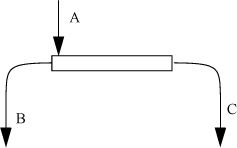
Inlet A is at 5 bar and 310 K and 3.2 mol/min. Outlet B is at 1 bar and 260 K. Outlet C is at 1 bar and 315 K. The tube is insulated and the fluid is air with CP = 7R/2.
a. Determine the flowrates of streams B and C.
b. Determine ![]() for the Hilsch tube.
for the Hilsch tube.
c. Suppose a reversible heat engine is connected between the outlet streams B and C which is run to produce the maximum work possible. The proposed heat engine may only exchange heat between the streams and not with the surroundings as shown. The final temperature of streams B and C will be TB′ as they exit the apparatus. What is TB′?
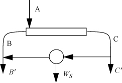
d. What work output is possible in W? What is ![]() for the entire system including the tube plus the heat engine?
for the entire system including the tube plus the heat engine?
e. Suppose that instead of using the heat engine, streams B and C were mixed directly with one another to form a single outlet stream. What would this temperature be, and how does it compare with TB′ from part (c)? Calculate ![]() and compare it with
and compare it with ![]() from part (c). What do you conclude from the comparison?
from part (c). What do you conclude from the comparison?
4.34. Methane gas is contained in a 0.65-m3 gas cylinder at 6.9 MPa and 300 K. The cylinder is vented rapidly until the pressure falls to 0.5 MPa. The venting occurs rapidly enough that heat transfer between the cylinder walls and the gas can be neglected, as well as between the cylinder and the surroundings. What is the final temperature and the final number of moles of gas in the tank immediately after depressurization? Assume the expansion within the tank is reversible, and the following:
a. Methane is considered to be an ideal gas with CP/R = 4.298
b. Methane is considered to be a real gas with properties given by a property chart.
4.35. A thermodynamically interesting problem is to analyze the fundamentals behind the product called “fix-a-flat.” In reality, this product is a 500 mL can that contains a volatile compound under pressure, such that most of it is liquid. Nevertheless, we can make an initial approximation of this process by treating the contents of the can as an ideal gas. If the initial temperature of both the compressed air and the air in the tire is 300 K, estimate the initial pressure in the compressed air can necessary to reinflate one tire from 1 bar to 3 bar. Also, estimate the final air temperature in the tire and in the can. For the purposes of this calculation you may assume: air is an ideal gas with CP/R = 7/2, the tire does not change its size or shape during the inflation process, and the inner tube of the tire has a volume of 40,000 cm3. We will reconsider this problem with liquid contents, after discussing phase equilibrium in a pure fluid.
4.36. Wouldn’t it be great if a turbine could be put in place of the throttle in problem 4.35? Then you could light a small bulb during the inflation to see what you were doing at night. How much energy (J) could possibly be generated by such a turbine if the other conditions were the same as in problem 4.35?
4.37. A 1 m3 tank is to be filled using N2 at 300 K and 20 MPa. Instead of throttling the N2 into the tank, a reversible turbine is put in line to get some work out of the pressure drop. If the pressure in the tank is initially zero, and the final pressure is 20 MPa, what will be the final temperature in the tank? How much work will be accomplished over the course of the entire process? (Hint: Consider the entropy balance carefully.)
4.38. Two well-insulated tanks are attached as shown in the figure below. The tank volumes are given in the figure. There is a mass-flow controller between the two tanks. Initially, the flow controller is closed. At t = 0, the mass flow controller is opened to a flow of 0.1 mol/s. After a time of 500 seconds, what are the temperatures of the two tanks? Neglect the heat capacity of the tanks and piping. No heat transfer occurs between the two tanks. (After 500 seconds, the pressure in the left tank is still higher than the pressure in the right tank.) The working fluid is nitrogen and the ideal gas law may be assumed. The ideal gas heat capacity CP = 7/2·R may be assumed to be independent of T.
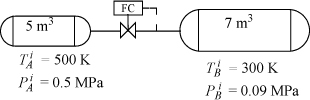
4.39. Two storage tanks (0.1 m3 each) contain air at 2 bar. They are connected across a small reversible compressor. The tanks, connecting lines, and compressor are immersed in a constant temperature bath at 280 K. The compressor will take suction from one tank, compress the gas, and discharge it to the other tank. The gas is at 280 K at all times. Assume that air is an ideal gas with CP = 29.3 J/mol-K.
a. What is the minimum work interaction required to compress the gas in one tank to 3 bar?
b. What is the heat interaction with the constant temperature bath?
4.40. A constant pressure air supply is connected to a small tank (A) as shown in the figure below. With valves B and C, the tank can be pressurized or depressurized. The initial conditions are T = 300 K, P = 1.013 bar, CP = 29.3 J/(mol-K). Consider the system adiabatic.
a. The tank is pressurized with valve B open and valve C closed. What is the final temperature of the tank? Neglect the heat capacity of the tank and valves.
b. Taking the system as the tank plus the valves, what is the entropy change of the system due to pressurization? What is the entropy change of the air supply reservoir? What is the entropy change of the universe? Use a reference state of 300 K and 1.013 bar.
c. During depressurization with valve B closed and valve C open, how does the molar entropy entering valve C compare with the molar entropy leaving? What is the temperature of the tank following depressurization?
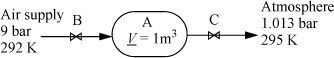
4.41. The pressurization of problem 4.40 is performed by replacing the inlet valve with a reversible device that permits pressurization that is internally reversible. The system is to remain adiabatic with respect to heat transfer of the surroundings.
a. What is the final temperature of the tank?
b. How much work could be obtained?
4.42. A 2m3 tank is at 292 K and 0.1 MPa and it is desired to pressurize the tank to 3 MPa. The gas is available from an infinite supply at 350 K and 5 MPa connected to the tank via a throttle valve. Assume that the gas follows the ideal gas law with a constant heat capacity of CP = 29 J/(mol-K).
a. Modeling the pressurization as adiabatic, what is the final temperature in the tank and the final number of moles when the pressure equals 3 MPa?
b. Identify factors included in the idealized calculation of part (a) that contribute to irreversibilities.
c. Identify factors neglected in the analysis of part (a) that would contribute to irreversibilities in a real process.
d. If the pressurization could be performed reversibly, the final temperature might be different from that found in part (a). Clearly outline a procedure to calculate the temperature indicating that enough equations are provided for all unknowns. Also clearly state how you would use the equations. Additional equipment is permissible provided that the process remains adiabatic with regard to heat transfer to the surroundings.
e. In part (d), would work be added, removed, or not involved in making the process reversible? Provide equations to calculate the work interaction.
4.43. Two gas storage tanks are interconnected through an isothermal expander. Tank 1 (V = 1 m3) is initially at 298 K and 30 bar. Tank 2 (V = 1 m3) is initially at 298 K and 1 bar. Reversible heat transfer is provided between the tanks, the expander, and the surroundings at 298 K. What is the maximum work that can be obtained from the expander when isothermal flow occurs from tank 1 to tank 2?