Chapter 15. Phase Equilibria in Mixtures by an Equation of State
The whole is simpler than the sum of its parts.
J.W. Gibbs
Suppose it was required to estimate the vapor-liquid K-ratio of methane in a mixture at room temperature. For an initial guess, we might assume it follows ideal-solution behavior. It is a relatively simple molecule (e.g., no polar moments, no hydrogen bonding). But we cannot use Raoult’s law because the required temperature is well above the critical temperature. We could use Henry’s law, or the SCVP+ model (Section. 11.12), but the assumption of low concentrations may be inappropriate at very high pressures. The equation of state method discussed here is an attractive alternative.
We begin this chapter with a review of the mixing rules introduced in Section 12.1. Then we show how the mixing rule leads to the fugacities and K-ratios needed for VLE calculations. We then provide algorithms and illustrate how VLE calculations are programmed using an equation of state (EOS). Finally we provide some insight into how critical behavior in mixtures differs from critical behavior in pure components, and that some “counterintuitive” behavior can exist, such as quality that decreases when pressure is increased.
Chapter Objectives: You Should Be Able to...
1. Compute VLE phase diagrams using an EOS.
2. Characterize adjustable parameters in EOS models using experimental data.
3. Derive an expression for a fugacity coefficient given an arbitrary EOS and mixing rules.
4. Comment critically on the merits and limitations of the PREOS relative to the activity models of Chapters 11–13, including the ability to suggest ways that the PREOS can be systematically improved.
15.1. Mixing Rules for Equations of State
Virial Equation of State
The virial equation was introduced for pure fluids in Section 7.4. Previously, we have also given a strategy for relating parameters to composition in Section 12.1. If we extend this mixing rule to the virial equation,

which for a binary mixture becomes
Similar to our previous discussion, it is understood that B12 is equivalent to B21. The cross coefficient B12 is not the virial coefficient for the mixture.
To obtain the cross coefficient, B12, we must create a combining rule to propose how the cross coefficient depends on the properties of the pure components 1 and 2. For the virial coefficient, the relationship between the pair potential and the virial coefficient was given in Section 7.11. However, a less rigorous method is often used in engineering applications. Rather, combining rules are created to use the corresponding state correlations developed for pure components in terms of Tc12 and Pc12. The combining rules used to determine the values of the cross coefficient critical properties are:
![]() Binary interaction parameters are used to adjust the combining rule to better fit experimental data, if available.
Binary interaction parameters are used to adjust the combining rule to better fit experimental data, if available.
The parameter k′12 is an adjustable parameter (called the binary interaction parameter) to force the combining rules to more accurately represent the cross coefficients found by experiment.1 However, in the absence of experimental data, it is customary to set k′12 = 0.
and
The first three of these combining rules lead to:
Then, Tc12, Pc12, and ω12 are used in the virial coefficient correlation presented in Chapter 7 to obtain B12 (Eqns. 7.6–7.10) which is subsequently incorporated into the equation for the mixture. If Zc (or Vc) is not available, it may be estimated using Zc = 0.291 – 0.08ω. The virial equation for a binary mixture is implemented on the spreadsheet Virialmx.xlsx furnished with the text.
Example 15.1. The virial equation for vapor mixtures
Calculate the molar volume for a 60 mole% mixture of neopentane(1) in CO2(2) at 310 K and 0.2 MPa.
Solution
The conditions are entered in the spreadsheet Virialmx.xlsx, with the following results:
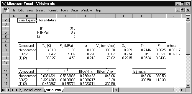
The original spreadsheet is modified slightly for this solution. Cells J9 and J10 are programmed with a rearranged form of Eqn. 7.10, Tr – 0.686 – 0.439Pr, and if these cells are positive, then the virial equation is suitable. The critical volume is calculated from Tc, Pc, and Zc. Cells F15–F17 list the virial coefficients for neopentane, CO2, and the cross coefficient, respectively.
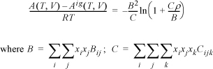
The virial coefficient for the mixture is given by Eqn. 15.1,
B = 0.62·(–846.06) + 2(0.6)(0.4)(–330.5) + 0.42·(–113.39) = –481.36 cm3/mol
V = RT/P + B = 8.314 · 310/0.2 – 481.36 = 12,405 cm3/mol
The volumetric behavior of the mixture depends on composition. The mixture volume differs from an ideal solution, ![]() . The difference V – Vis is called the excess volume, VE.
. The difference V – Vis is called the excess volume, VE.
The molar volume of pure neopentane is
V = RT/P + B = 8.314 · 310/0.2 – 846.1 = 12,041 cm3/mol
The molar volume of pure CO2 is
V = RT/P + B = 8.314 · 310/0.2 – 113.4 = 12,773 cm3/mol
The molar volume of an ideal solution of a 60 mole% neopentane mixture is
Vis = 0.6(12,041) + 0.4(12,773) = 12,334 cm3/mol
and the excess volume is
VE = 12,405 – 12,334 = 71.2 cm3/mol.
The molar volume and excess volume can be determined across the composition range by changing y’s in the formulas.
Cubic Equations of State
The customary mixing rules for cubic equations of state have been introduced in Section 12.1:
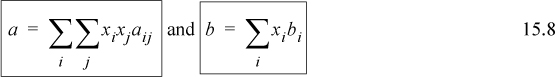
Note the mathematical similarity of the mixing rule for a with the mixing rule used for the virial coefficient. All of the compositional dependence of the equation of state is incorporated into the two relations. A combining rule is not necessary for the b term, however the a term does require a combining rule. The customary combining rule is
where kij is referred to as a binary interaction parameter. This is similar to the form of the geometric mean rule for critical temperatures used for virial coefficients. The adjustable parameter kij is used to adjust the combining rule to fit experimental data more closely. Technically, this just transfers our ignorance into the adjustable parameter kij. Values for kij for various binary combinations are tabulated in the literature.2
In the absence of experimental data or literature values for kij, we may make a first-order approximation by letting kij = 0. This approximation serves our purpose nicely, because the equation of state approach then requires no more information than the ideal solution approach (Tc, Pc, ω, T, P, x, y), but it offers the possibility of more realistic representation of the phase diagram because of the more fundamental molecular basis. We can demonstrate this improved accuracy by considering some examples.
![]() Review of the concepts from Section 10.8 may help put the approaches in context. Keep in mind that the objective is still to perform bubble, dew and flash calculations, but after relaxing the ideal solution assumption.
Review of the concepts from Section 10.8 may help put the approaches in context. Keep in mind that the objective is still to perform bubble, dew and flash calculations, but after relaxing the ideal solution assumption.
15.2. Fugacity and Chemical Potential from an EOS
We begin with a reminder that for phase equilibria calculations, that the fugacities of components are needed. The tool that we need for VLE calculations is the K-ratio and an expression for the component fugacity. In Section 10.9 we demonstrated that the component fugacity for an ideal gas component is equal to the partial pressure. In this chapter we develop a method of “correcting” the partial pressure to provide the fugacity. As a variation of the Venn diagram presented in Fig. 11.8, we present the schematic shown in Fig. 15.1. Because the equation of state is capable of representing liquid phases by using the smaller root, we show both vapor and liquid phases.

Figure 15.1. Schematic showing the equation of state approach to modeling fugacities of components. Departure function (fugacity coefficient) methods are used for both the vapor and liquid phases. Superscripts are used to distinguish the fugacity coefficients of each phase. Liquid-phase compositions are conventionally denoted by xi and vapor-phase compositions by yi.
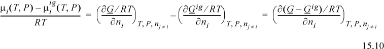
The method of deriving the fugacity is an extension of Eqn. 10.39. If we compare the chemical potential in the real mixture to the chemical potential for an ideal gas, we see that the difference is given by the component derivative of the Gibbs departure.
We have seen the Gibbs departure in Eqns. 9.23 and 9.31. For the virial equation, we have
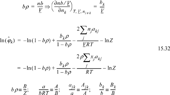
where we recognize that the virial coefficient depends on composition via Eqn. 15.2. By differentiation of this expression, we obtain the chemical potential. We can calculate the component fugacity if we use Eqn. 11.22 and replace the standard state with the ideal gas mixture state. Since the component fugacity in the ideal gas state is the partial pressure, the fugacity coefficient becomes
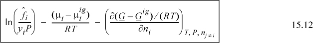
We define the ratio of the component fugacity to the partial pressure (ideal gas component fugacity) as the component fugacity coefficient.

Differentiation of the Gibbs departure leads to the component fugacity coefficients for a binary,
which will be shown in more detail later. The fugacity coefficient of a component in a mixture may be directly determined at a given T and P by evaluating the virial coefficients at the temperature, then using this equation to calculate the fugacity coefficient.
Differentiation of the Gibbs departure function is difficult for a pressure-explicit equation of state like the Peng-Robinson equation of state. The difficulty arises because the Gibbs departure function is given in terms of volume and temperature rather than pressure (Eqns. 8.36 and 9.33), and differentiation at constant pressure as required by Eqn. 15.12 is difficult. As in the case of pure fluids, classical thermodynamics provides the means to solve this problem. Instead of differentiating the Gibbs departure function, we differentiate the Helmholtz departure function. Recalling,
and noting,
we also use A = G – PV, or dA = dG – d(PV):

Equating coefficients of dni we see an alternative method to find the chemical potential,
Note that T, P, and V identify the same conditions for the real fluid. Therefore, when we evaluate the departure, the ideal gas state must be corrected from Vig to V,
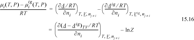
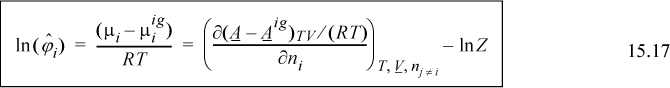
where the notation (A – Aig)TV denotes a departure function at the same T, V, which is the integral of Eqn. 8.27. The last term, ln Z, represents the correction of the ideal gas Helmholtz energy from V to Vig. Careful inspection of the true form on the integral leading to ln Z should convince you that differentiation does not change this term, and only the integral for the departure in Eqn. 15.16 must be differentiated.
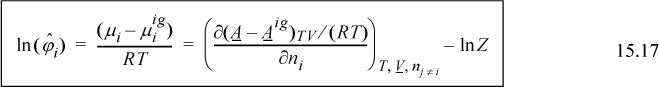
![]() General form for fugacity coefficient for a pressure explicit equation of state such as the Peng-Robinson, that is, Z(T,ρ).
General form for fugacity coefficient for a pressure explicit equation of state such as the Peng-Robinson, that is, Z(T,ρ).
Therefore, the fugacity coefficient is calculated using
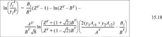
To apply this, consider the Peng-Robinson equation as an example.

By extending the method of reducing the equation of state parameters developed in Eqns. 7.21 and 7.22, ![]() and
and ![]() , where
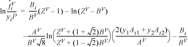
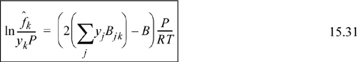
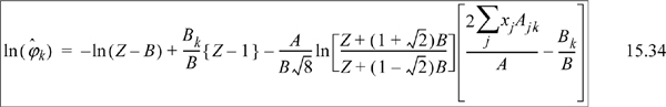
, where ![]() . Then, differentiation as we will show in Example 15.5 on page 592, yields for a binary system
. Then, differentiation as we will show in Example 15.5 on page 592, yields for a binary system
As we saw in the case of equations of state for pure fluids, there is no fundamental reason to distinguish between the vapor and liquid phases except by the magnitude of Z. The equation of state approach encompasses both liquids and vapors very simply. We replace the vapor phase mole fractions with liquid phase mole fractions in all formulas including those for A and B, resulting in
Recalling that ![]() at equilibrium, we write the equality and rearrange to find the expression for the K-ratio used to solve VLE problems.
at equilibrium, we write the equality and rearrange to find the expression for the K-ratio used to solve VLE problems.

![]() Eqn. 15.20 provides the primary equations for VLE via equations of state. Different equations of state provide different formulas for
Eqn. 15.20 provides the primary equations for VLE via equations of state. Different equations of state provide different formulas for ![]() .
.
Given Ki for all i, it is straightforward to solve VLE problems using the same procedures as for ideal solutions.
Note: Eqns. 15.20 provide the primary equations for VLE via equations of state. These equations are implemented by iteration procedures summarized in Appendix C. Only the bubble method will be presented in the chapter in detail. Although cubic equations can represent both vapor and liquid phases, note that the virial equation cannot be used for liquid phases.
Bubble-Pressure Method
For a bubble-pressure calculation, the T and all xi are known as shown in Table 10.1 on page 373. Like the simple calculation performed in the preceding chapter, the criterion for convergence is ![]() which needs to be expressed in terms of variables for the current method. Rearranging Eqn. 15.20, this sum becomes
which needs to be expressed in terms of variables for the current method. Rearranging Eqn. 15.20, this sum becomes 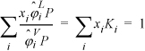 . Unlike the activity model calculations, we cannot explicitly solve for pressure because all
 ![]() and
and ![]() depend on pressure. Additionally,
depend on pressure. Additionally, ![]() all depend on composition of the vapor phase, which is not exactly known until the problem is solved. Typically, we use Raoult’s law with the shortcut vapor pressure equation for the first guesses of yi and P. From these values, we determine all Ki and check the sum of y values. If the sum is greater than one, the pressure guess is increased, if less than one, the pressure guess is decreased. A complete flowchart and example will be discussed in Section 15.4, but for now, let us explore the methods for calculating the fugacity coefficients.
all depend on composition of the vapor phase, which is not exactly known until the problem is solved. Typically, we use Raoult’s law with the shortcut vapor pressure equation for the first guesses of yi and P. From these values, we determine all Ki and check the sum of y values. If the sum is greater than one, the pressure guess is increased, if less than one, the pressure guess is decreased. A complete flowchart and example will be discussed in Section 15.4, but for now, let us explore the methods for calculating the fugacity coefficients.
As we observed for pure fluids, it is important to select the proper root when applying an equation of state. Considering the Workbook Prfug.xlsx, for the one-root region, we should select that row for the fugacity coefficients. For the three-root region, we should choose the root with the lowest mixture fugacity. At low pressure and near room temperature, systems are usually in the three-root region for both liquid and vapor compositions, but that may change as we approach the critical region. The number of roots depends on composition as well as T and P. For example, it often occurs that one root occurs using the vapor composition when one component is supercritical in equilibrium with a liquid phase. This means we need to select among at least four possibilities for each phase when computing the K-values: largest Z root for vapor composition, smallest Z root with liquid composition, single root with vapor composition, single root with liquid composition. If we compute K-values with all four ratios, only one of the possibilities provides meaningful results and these are the ones to apply in the next iteration.
Example 15.2. K-values from the Peng-Robinson equation
The bubble-point pressure of an equimolar nitrogen (1) + methane (2) system is to be calculated by the Peng-Robinson equation and compared to the shortcut K-ratio estimate at 100 K. The shortcut K-ratio estimate will be used as an initial guess: P = 0.4119 MPa, yN2 = 0.958. Apply the formulas for the fugacity coefficients to obtain an estimate of the K-values for nitrogen and methane and evaluate the sum of the vapor mole fractions based on this initial guess.
Solution
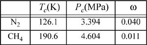
The spreadsheet Prfug.xlsx may be used to follow the calculations. The K-values using the vapor root with vapor composition and liquid root with liquid composition are valid throughout the iterations of this example. From the shortcut calculation, P = 0.4119 MPa at 100 K. Applying Eqns. 7.21 and 7.22 for the pure component parameters:
For N2: A11 = 0.09686; B1 = 0.011906;
For CH4: A22 = 0.18242; B2 = 0.013266
By the square-root combining rule Eqn. 15.9: A12 = 0.13293
Based on the vapor composition of the shortcut estimate at y1 = 0.958, the mixing rule gives AV = 0.099913; BV = 0.01196; Solving the cubic for the vapor root at this composition gives ZV = 0.9059.
Then

Many of the terms are the same for the methane in the mixture:
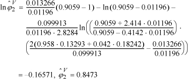
To save some tedious calculations, the liquid formulas have already been applied to obtain: ![]() ;
; ![]() . Determining the K values,
. Determining the K values,
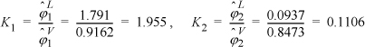
y1 = 0.5 · 1.955 = 0.978; y2 = 0.5 · 0.1106 = 0.055; ![]()
A higher guess for P would be appropriate for the next iteration in order to make the K-values smaller. ![]() and
and ![]() would need to be evaluated at the new pressure. The calculations are obviously tedious. Ki calculations are possible in Excel by first copying the “Fugacities” sheet on Prfug.xlsx, using one sheet for liquid and the other for vapor, and then referencing cells on one of the sheets to calculate the Ki. We provide an example of such an arrangement in Prmix.xlsx. More details on the entire procedure will follow in Section 15.4.
would need to be evaluated at the new pressure. The calculations are obviously tedious. Ki calculations are possible in Excel by first copying the “Fugacities” sheet on Prfug.xlsx, using one sheet for liquid and the other for vapor, and then referencing cells on one of the sheets to calculate the Ki. We provide an example of such an arrangement in Prmix.xlsx. More details on the entire procedure will follow in Section 15.4.
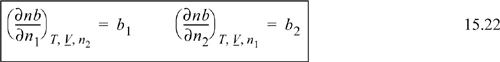
15.3. Differentiation of Mixing Rules
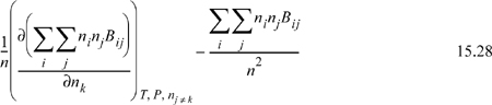
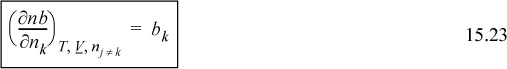
Since a compositional derivative is necessary to obtain the partial molar quantities, and the compositions are present in summation terms, we must understand the procedures for differentiation of the sums. Since all of the compositional dependence is embedded in these terms, if we understand how these terms are handled, we can then apply the results to any equation of state. Only three types of sums appear in most forms of equations of state, which have been introduced above. The first type of derivative we will encounter is of the form
![]() Since the compositional dependence is within the mixing rule, if we understand how to differentiate the general mixing rules, then we can easily apply them to the models that use them.
Since the compositional dependence is within the mixing rule, if we understand how to differentiate the general mixing rules, then we can easily apply them to the models that use them.
where ![]() . For a binary nb = n1b1 + n2b2, and k will be encountered once in the sum, whether k = 1 or k = 2, thus:
. For a binary nb = n1b1 + n2b2, and k will be encountered once in the sum, whether k = 1 or k = 2, thus:
and the general result is

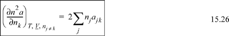
The second type of derivative which we will encounter is of the form
n2a may be written as ![]() . For a binary mixture,
. For a binary mixture, ![]() . Taking the appropriate derivative,
. Taking the appropriate derivative,
The general result is
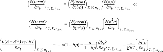
For the virial equation, we need to differentiate a function that will look like:

Differentiation by the product rule gives
The double sum in the derivative is n2B which we have evaluated in equivalent form in Eqn. 15.25. The second term is just B given by Eqn. 15.1. Therefore, we have for a binary mixture

The general result is

Example 15.3. Fugacity coefficient from the virial equation
For moderate deviations from the ideal-gas law, a common method is to use the virial equation given by:
Z = 1 + BP/RT
where ![]() . Develop an expression for the fugacity coefficient.
. Develop an expression for the fugacity coefficient.
Solution
For the virial equation, we have the result of Eqn. 9.30, ![]()
Applying Eqn. 15.12

the argument we need to differentiate looks like ![]() .
.
Differentiation has been performed in Eqn. 15.29, which we can generalize as
which has been shown earlier for a binary in Eqn. 15.14.
Example 15.4. Fugacity coefficient from the van der Waals equation
Van der Waals’ equation of state provides a simple but fairly accurate representation of key equation of state concepts for mixtures. The main manipulations developed for this equation are the same for other equations of state but the algebra is a little simpler. Recalling van der Waals’ equation from Chapter 6,
where ![]() and
and ![]() . Develop an expression for the fugacity coefficient.
. Develop an expression for the fugacity coefficient.
Solution
We need to apply Eqn. 15.17. For the departure, we apply Eqn. 8.27 because the differentiation indicated above is performed at constant volume, not constant pressure.
Apply Eqn. 15.17, but instead of differentiating directly, use the chain rule, Eqn. 6.16.
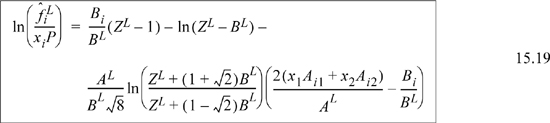
Example 15.5. Fugacity coefficient from the Peng-Robinson equation
The Peng-Robinson equation is given by
where ![]() and
and ![]() . Develop an expression for the fugacity coefficient.
. Develop an expression for the fugacity coefficient.
Solution
We need to apply Eqn. 15.17. From integration for the pure fluid,

The next steps look intimidating. Basically, they apply the same procedure for differentiation as the last example.
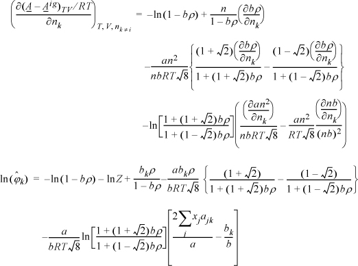
Note a simplification that is not obvious:
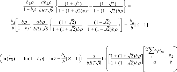
Substituting the following definitions,
which has been shown in Eqns. 15.18–15.19 for a binary.
15.4. VLE Calculations by an Equation of State
At the end of Section 15.2, the bubble-pressure method was briefly introduced to show how the fugacity coefficients are incorporated into a VLE calculation, without concentrating on the details of the iterations. Section 15.3 offered derivations of formulas for the fugacity coefficients that were presented without proof at the beginning of the chapter. Now, it is time to turn to the applied engineering objective: calculation of phase equilibria. Refer again to Table 10.1 on page 373, that lists the types of routines that are needed and the convergence criteria. Note that Table 10.1 is independent of the model used for calculating VLE. As an example of the iteration procedure for cubic equations of state, the bubble-pressure flow sheet is presented in Fig. 15.2. The flow sheet puts detail to the procedure discussed superficially in Example 15.2 and immediately preceding the example. Flow sheets for bubble temperature, dew, and flash routines are available in Appendix C. As with ideal solutions, the bubble-pressure routine is the easiest to apply, so we cover it in detail in the following examples. Iterative phase equilibrium calculations can be tedious and difficult to automate. We can facilitate the calculations to some extent by combining two copies of the PrFug spreadsheet into a single workbook, which we call Prmix.xlsx. The four possible K-value representations are included for convenient selection, as described in Example 15.2. This workbook forms only a starting basis with an emphasis on clearly showing the fundamental steps.
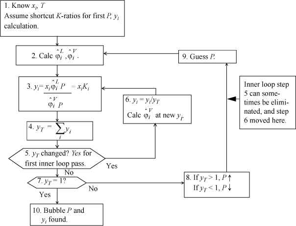
Figure 15.2. Bubble-pressure flow sheet for the equation of state method of representing VLE. Other routines are given in Appendix C.
Example 15.6. Bubble-point pressure from the Peng-Robinson equation
Use the Peng-Robinson equation (kij = 0) to determine the bubble-point pressure of an equimolar solution of nitrogen (1) + methane (2) at 100 K.
Solution
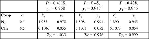
The calculations proceed by first calculating the short-cut K-ratio as in Example 15.2 on page 587. The ideal-solution (is) bubble pressure was ![]() ; yN2is = 0.958. In fact, the K-values for the first iteration have already been determined in that example, in great detail. The values from that example are K1 = 1.955, K2 = 0.1106. The new estimates of vapor mole fractions are obtained by multiplying xi·Ki. In Example 15.2, the sum was found to be
; yN2is = 0.958. In fact, the K-values for the first iteration have already been determined in that example, in great detail. The values from that example are K1 = 1.955, K2 = 0.1106. The new estimates of vapor mole fractions are obtained by multiplying xi·Ki. In Example 15.2, the sum was found to be ![]() . These calculations are summarized in the first column of Table 10.1.
. These calculations are summarized in the first column of Table 10.1.
Noting that these sum to a number greater than unity, we must choose a greater value of pressure for the next iteration. Before we can start the next iteration, however, we must develop new estimates of the vapor mole fractions; the ones we have do not make sense because they sum to more than unity. These new estimates can be obtained simply by dividing the given vapor mole fractions by the number to which they sum. This process is known as normalization of the mole fractions. For example, to start the second iteration, y1 = 0.978/1.033 = 0.947. After repeating the process for the other component, the mole fractions will sum to unity. Since the result for the second iteration is less than one, the pressure guess is too high.
The third iteration consists of applying the interpolation rule to obtain the estimate of pressure and use of the normalization procedure to obtain the estimates of vapor mole fractions. P = 0.4119 + (1 – 1.033)/(0.956 – 1.033) · (0.45 – 0.4119) = 0.428 MPa. Since the estimated vapor mole fractions after the third iteration sum very nearly to unity, we may conclude the calculations here. This is the bubble pressure. Note how quickly the estimate for y1 converges to the final estimate of 0.945.
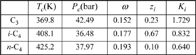
Example 15.7. Isothermal flash using the Peng-Robinson equation
A distillation column is to produce overhead products having the following compositions:
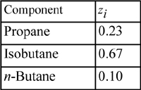
Suppose a partial condenser is operating at 320 K and 8 bars. What fraction of liquid would be condensed according to the Peng-Robinson equation, assuming all binary interaction parameters are zero (kij = 0)?
Solution
This is an isothermal flash calculation. Refer back to the same problem (Example 10.1 on page 382) for an initial guess based on the shortcut K-ratio equation. V/F = 0.25 ⇒ {xi} = {0.1829, 0.7053, 0.1117} and {yi} = {0.3713, 0.5642, 0.0648}. Substituting these composition estimates for the vapor and liquid compositions into the routine for estimating K-values (cf. Example 15.2 on page 587), we can obtain the estimates for K-values given below:
The computations for the flash calculation are basically analogous to those in Example 10.1, except that Ki values are calculated from Eqn. 15.20. A detailed flow sheet is presented in Appendix C. For this example, the K-values are not modified until the iteration on V/F converges. After convergence on V/F, the vapor and liquid mole fractions are recomputed using Eqns. 10.15 and 10.16, followed by recomputed estimates for the K-values. If the new estimates for K-values are equal to the old estimates for K-values, then the overall iteration has converged. If not, then the new estimates for K-values are substituted for the old values, and the next iteration proceeds just like the last. This method of iteratively solving for the vector of K-values is known in numerical analysis as the “successive substitution” method.
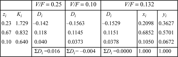
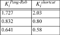
Using these x’s and y’s for guesses we find K = 1.7276, 0.8318, and 0.6407, respectively. These K-values are similar to those estimated at the compositions derived from the ideal-solution approximation, and will yield a similar V/F. Therefore, we conclude that this iteration has converged (a general criterion is that the average % change in the K-values from one iteration to the next is less than 10-4). Comparison to the shortcut K-ratio approximation shows small but significant deviations—V/F = 0.13 for Peng-Robinson versus 0.25 for the shortcut K-ratio method.
Based on this example, we may conclude that the shortcut K-Ratio approximation provides a reasonable first approximation at these conditions. Note, however, that none of the components is supercritical and all the components are saturated hydrocarbons.
It is tempting to expand further on Prmix.xlsx to facilitate greater automation and simple-minded application. An online supplement provides a very preliminary step in this direction through the use of macro’s. Ultimately, however, this literature comprises specialized research that is beyond our introductory scope. In general, the analysis requires detailed consideration of phase stability and criticality. References cited in Chapter 16 describe works by Michelsen and Mollerup, Eubank, and Tang that can help to create more reliable algorithms. It is a useful exercise to customize your workbooks to increase your confidence in achieving reliable solutions, but do not spend excessive time trying to program every possibility. Chapter 16 and the references cited there are recommended for advanced programming.
Example 15.8. Phase diagram for azeotropic methanol + benzene
Methanol and benzene form an azeotrope. For methanol + benzene the azeotrope occurs at 61.4 mole% methanol and 58°C at atmospheric pressure (1.01325 bars). Additional data for this system are available in the Chemical Engineers’ Handbook. Use the Peng-Robinson equation with kij = 0 (see Eqn. 15.9) to estimate the phase diagram for this system and compare it to the experimental data on a T-x-y diagram. Determine a better estimate for kij by iterating on the value until the bubble point pressure matches the experimental value (1.013 bar) at the azeotropic composition and temperature. Plot these results on the T-x-y diagram as well. Note that it is impossible to match both the azeotropic composition and pressure with the Peng-Robinson equation because of the limitations of the single parameter, kij.
The experimental data for this system are as follows:

Solution
Solving this problem is computationally intensive, but still approachable with Prmix.xlsx. The strategy is to manually set a guessed kij and then perform a bubble pressure calculation at the azeotrope temperature (331.15 K) and composition, xm = 0.614. The program will give a calculated pressure and vapor phase composition. The vapor-phase composition may not match the liquid-phase composition because the azeotrope is not perfectly predicted; however, we continue to manually change kij, and repeat the bubble pressure calculation until we match the experimental pressure of 1.013 bar. The following values are obtained for the bubble pressure at the experimental azeotropic composition and temperature with various values of kij.
The resultant kij is used to perform bubble-temperature calculations across the composition range, resulting in Fig. 15.3. Note that we might find a way to fit the data more accurately than the method given here, but any improvements would be small relative to estimating kij = 0. We see that the fit is not as good as we would like for process design calculations. This solution is so nonideal that a more flexible model of the thermodynamics is necessary. Note that the binary interaction parameter alters the magnitude of the bubble-pressure curve very effectively but hardly affects the skewness at all. Since this mixture is far from the critical region, a two-parameter activity model like van Laar or UNIQUAC would be recommended as shown in Fig. 12.1. The Peng-Robinson model with van der Waals’ mixing rule comes closest to the Scatchard-Hildebrand activity model. We observed that the Scatchard-Hildebrand model performed poorly for hydrogen bonding mixtures. Two approaches are common when precision is needed in the critical region for hydrogen bonding mixtures. Either a multiparameter activity model can be adapted as a basis for an advanced mixing rule, or hydrogen bonding can be treated explicitly. References to these are approaches are presented in the chapter summary.
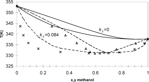
Figure 15.3. T-x-y diagram for the azeotropic system methanol + benzene. Curves show the predictions of the Peng-Robinson equation (kij = 0) and correlation (kij = 0.084) based on fitting a single data point at the azeotrope; x’s and triangles represent liquid and vapor phases, respectively.
Example 15.9. Phase diagram for nitrogen + methane
Use the Peng-Robinson equation (kij = 0) to determine the phase diagram of nitrogen + methane at 150 K. Plot P versus x, y and compare the results to the results from the shortcut K-ratio equations.
Solution
First, the shortcut K-ratio method gives the dotted phase diagram in Fig. 15.4. Applying the bubble-pressure procedure with the program Prmix.xlsx, we calculate the solid line in Fig. 15.4. For the Peng-Robinson method we assume K-values from the previous solution as the initial guess to get the solutions near xN2 = 0.685. The program Prmix.xlsx assumes this automatically, but we must also be careful to make small changes in the liquid composition as we approach the critical region.
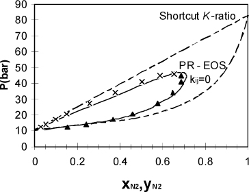
Figure 15.4. High pressure P-x-y diagram for the nitrogen + methane system comparing the shortcut K-ratio approximation and the Peng-Robinson equation at 150 K. The data points represent experimental results. Both theories are entirely predictive since the Peng-Robinson equation assumes that kij = 0.
Fig. 15.4 was generated by entering liquid nitrogen compositions of 0.10, 0.20, 0.40, 0.60, 0.61, 0.62..., 0.68, and 0.685. This procedure of starting in a region where a simple approximation is reliable and systematically moving to more difficult regions using previous results is often necessary and should become a familiar trick in your accumulated expertise on phase equilibria in mixtures. We apply a similar approach in estimating liquid-liquid equilibria.
Comparing the two approximations numerically and graphically, it is clear that the shortcut approximation is significantly less accurate than the Peng-Robinson equation at high concentrations of the supercritical component. This happens because the mixture possesses a critical point, above which separate liquid and vapor roots are impossible, analogous to the situation for pure fluids. Since the mixing rules are in terms of a and b instead of Tc and Pc, the equation of state is generating effective values for Ac and Bc of the mixture.
Instead of depending simply on T and P as they did for pure fluids, however, Ac and Bc also depend on composition. The mixture critical point varies from one component to the other as the composition changes. Since the shortcut (and also SCVP+) approximation extrapolates the vapor pressure curve to obtain an effective vapor pressure of the supercritical component, that approximation does not reflect the presence of the mixture critical point and this leads to significant errors as the mixture becomes rich in the supercritical component.
The mixture critical point also leads to computational difficulties. If the composition is excessively rich in the supercritical component, the equation of state calculations may obtain the same solution for the vapor root as for the liquid root and, since the fugacities are equal, the program will terminate. The program may indicate accurate convergence in this case due to some slight inaccuracies that are unavoidable in the critical region. Or the program may diverge. It is often up to the competent engineer to recognize the difference between accurate convergence and a spurious answer. Plotting the phase envelope is an excellent way to stay out of trouble.
![]() The shortcut K-ratio method provides an initial estimate when a supercritical component is at low liquid-phase compositions, but incorrectly predicts VLE at high liquid-phase concentrations of the supercritical component.
The shortcut K-ratio method provides an initial estimate when a supercritical component is at low liquid-phase compositions, but incorrectly predicts VLE at high liquid-phase concentrations of the supercritical component.
Example 15.10. Ethane + heptane phase envelopes
Use the Peng-Robinson equation (kij = 0) to determine the phase envelope of ethane + n-heptane at compositions of xC7 = [0, 0.1, 0.2, 0.3, 0.5, 0.7, 0.9, 1.0]. Plot P versus T for each composition by performing bubble-pressure calculations to their terminal point and dew-temperature calculations until the temperature begins to decrease significantly and the pressure approaches its maximum. If necessary, close the phase envelope by starting at the last dew-temperature state and performing dew-pressure calculations until the temperature and pressure approach the terminus of the bubble-point curve. For each composition, mark the points where the bubble and dew curves meet with X’s. These X’s designate the “mixture critical points.” Connect the X’s with a dashed curve. The dashed curve is known as the critical locus of the mixture.
Solution
Note that these phase envelopes are similar to the one from the previous problem, except that we are changing the temperature instead of the composition along each curve. They are more tedious in that both dew and bubble calculations must be performed to generate each curve. The lines of constant composition are sometimes called isopleths. The results of the calculations are illustrated in Fig. 15.5. The results at mole fractions of 0 and 1.0 are indicated by dash-dot curves to distinguish them as the vapor pressure curves. Phase equilibria on the P-T plot occurs at the conditions where a bubble line of one composition intersects a dew line of a different composition.
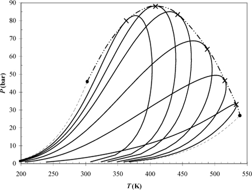
Figure 15.5. High pressure phase envelopes for the ethane + heptane system comparing the effects of composition according to the Peng-Robinson equation. The theory is entirely predictive because the Peng-Robinson equation has been applied with kij = 0. X’s mark the mixture critical points and the dashed line indicates the critical locus. The first and last curves represent the vapor pressures for the pure components.
Some practical considerations for high pressure processing can be inferred from the diagram. Consider what happens when starting at 90 bars and ~445 K and dropping the pressure on a 30 mole% C7 mixture at constant temperature. Similar situations could arise with flow of natural gas through a small pipe during natural gas recovery. As the pressure drops, the dew-point curve is crossed and liquid begins to condense. Based on intuition developed from experiences at lower pressure, one might expect that dropping the pressure should result in more vapor-like behavior, not condensation. On the other hand, dropping the pressure reduces the density and solvent power of the ethane-rich mixture. This phenomenon is known as retrograde condensation. It occurs near the critical locus when the operating temperature is less than the maximum temperature of the phase envelope. Since this maximum temperature is different from the mixture critical temperature, it needs a distinctive name. The name applied is the “critical condensation temperature” or cricondentherm. Similarly, the maximum pressure on the phase envelope is known as the cricondenbar. Note that an analogous type of phase transition can occur near the critical locus when the pressure is just above the critical locus and the temperature is changed.
To extend the analysis, imagine what happens in a natural gas stream composed primarily of methane but also containing small amounts of components as heavy as C80. A retrograde condensation region exists where the heavy components begin to precipitate, as discussed in Example 14.12 on page 567. But a different possibility also exists because the melting temperature of the heavy components may often exceed the operating temperature, and the precipitate that forms might be a solid that could stick to the walls of the pipe. This in turn generates a larger constriction which generates a larger pressure drop during flow, right in the vicinity of the deposit. In other words, this deposition process may tend to promote itself until the flow is substantially inhibited. Wax deposition is a significant problem in the oil and natural gas industry and requires considerable engineering expertise because it often occurs away from critical points, as well as in the near-critical regions of this discussion. A wide variety of solubility behavior can occur, as we show in Chapter 16.
15.5. Strategies for Applying VLE Routines
For some problems, such as generation of a phase diagram, the examples in this chapter can be followed directly. Often, however, it takes some thought to decide which type of VLE routine is appropriate to apply in a given situation. Do not discount this step in the problem solution strategy. Part of the objective of the homework problems is to increase understanding of phase behavior by encouraging thought about which routine to use. Since the equation of state routines are complicated enough to require a computer, they are also solved relatively rapidly, once the VLE routine has been identified. Use Table 10.1 on page 373 and the information in Section 10.1 to identify the correct procedure to apply before turning to computational techniques. Use the problem statement to identify whether the liquid, vapor, or overall mole fractions are known. Study the problem statement to see whether the P and T are known. Often this information together with Table 10.1 will determine the routines to apply. Sometimes more than one approach is satisfactory. Sometimes the ideal-solution approximation may be applied, and a review of Section 10.8 may be helpful. Before using software that accompanies the text, be sure to read the appropriate section of Appendix A, and the instructions or readme.txt files that accompany the program.
15.6. Summary
The essence of the equation of state approach to mixtures is that the equation of state for mixtures is the same as the equation of state for pure fluids. The expressions for Z, A, and U are exactly the same. The only difference is that the parameters (e.g., a and b of the Peng-Robinson equation) are dependent on the composition. That should come as no large surprise when you consider that these parameters must transform from pure component to pure component in some continuous fashion as the composition changes. What may be surprising is the wealth of behaviors that can be inferred from some fairly simple rules for modeling this transformation. Everything from azeotropes to retrograde condensation, and even liquid-liquid separation can be represented with qualitative accuracy based on this simple extension of the equation of state.
So, are we done with phase behavior modeling? Unfortunately, the keyword in the preceding paragraph is “qualitative.” Equations of state are sufficiently accurate for most applications involving hydrocarbons, gases, and to some extent, ethers, esters, and ketones. For many oil and gas wells, it may suffice to treat the hydrocarbon-rich phases in this way and treat water separately. But any applications involving strongly hydrogen-bonding species tend to require greater accuracy than currently attainable from equations like the Peng-Robinson EOS. For example, if methanol is used as a hydrate inhibitor in a gas well, its partitioning may require a more sophisticated treatment. One idea is to adapt multiparameter activity models like the UNIQUAC model as the basis for mixing rules. This is the approach of the Wong-Sandler model.3 Another approach is to analyze hydrogen bonding as simultaneous reaction and phase equilibria, as discussed in Chapter 19.
Important Equations
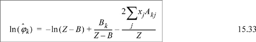
Once again the mixing rules play an important role in defining the thermodynamics. Since the Peng-Robinson mixing rules have the same form as the van der Waals mixing rules, including a single binary interaction parameter, kij, the Peng-Robinson model cannot match the skewness of the Gibbs excess curve, only the magnitude. Outside the critical region, you might as well use an activity model. The advantage of the Peng-Robinson model is that it provides a holistic framework that applies seamlessly to vapor, liquid, and critical region. Noting how activity models artificially designate different methods for different phases, it is gratifying to see that such conceptual simplicity is feasible. The key equation for establishing this feasibility is deriving the fugacity coefficient for a pressure-explicit equation of state:
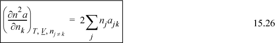
Given this equation, it is straightforward to derive fugacity coefficients, and K-ratios, for any equation of state or mixing rule. Two related equations that often appear are Eqns. 15.23 and 15.26.
Look for ways to rearrange the equations before differentiating such that these terms appear and then differentiation becomes much simpler, often reducing to simple substitution. Finally, the EOS method melds with every other phase equilibrium computational procedure when the expression is derived for the partition coefficient, as given by a slight variation on Eqn. 15.20.
Here we have generalized Eqn. 15.20 slightly by recognizing that the upper phase could be vapor or it could be the upper phase of LLE. The beauty of the EOS perspective is that the fluid phase model is the same for liquid or vapor; only the proper root must be selected.
15.7. Practice Problems
P15.1. Repeat all the practice problems from Chapter 10, this time applying the Peng-Robinson equation.
P15.2. Acrolein (C3H4O) + water exhibits an atmospheric (1 bar) azeotrope at 97.4 wt% acrolein and 52.4°C. For acrolein: Tc = 506 K; Pc = 51.6 bar; and ω = 0.330; MW = 56.
a. Determine the value of kij for the Peng-Robinson equation that matches this bubble pressure at the same liquid composition and temperature. (ANS. 0.015)
b. Tabulate P, y at 326.55 K and x = {0.57, 0.9, 0.95, 0.974} via the Peng-Robinson equation using the kij determined above. (ANS. (1.33, 0.575), (1.16, 0.736), (1.06, 0.841), (1.0, 0.860))
P15.3. Laugier and Richon (J. Chem. Eng. Data, 40:153, 1995) report the following data for the H2S + benzene system at 323 K and 2.010 MPa: x1 = 0.626; y1 = 0.986.
a. Quickly estimate the vapor-liquid K-value of H2S at 298 K and 100 bar. (ANS. 0.21)
b. Use the data to estimate the kij value, then estimate the error in the vapor phase mole fraction of H2S. (ANS. 0.011, 0.1%)
P15.4. The system ethyl acetate + methanol forms an azeotrope at 27.8 mol% EA and 62.1°C. For ethyl acetate, Tc = 523.2 K; Pc = 38.3 bar; and ω = 0.362.
a. What is the estimate of the bubble-point pressure from the Peng-Robinson equation of state at this composition and temperature when it is assumed that kij = 0? (ANS. 0.98 bars)
b. What value of kij gives a bubble-point pressure of 1 bar at this temperature and composition? (ANS. 0.0054)
c. What is the composition of the azeotrope and value of the bubble-point pressure at the azeotrope estimated by the Peng-Robinson equation when the value of kij from part (b) is used to describe the mixture? (ANS. xEA = 0.226)
a. Assuming zero for the binary interaction parameter (kij = 0) of the Peng-Robinson equation, predict whether an azeotrope should be expected in the system CO2 + ethylene at 222 K. Estimate the bubble-point pressure for an equimolar mixture of these components. (ANS. No, 8.7 bar)
b. Assuming a value for the binary interaction parameter (kij = 0.11) of the Peng-Robinson equation, predict whether an azeotrope should be expected in the system CO2 + ethylene at 222 K. Estimate the bubble-point pressure for an equimolar mixture of these components. (ANS. Yes, 11.3 bar)
a. Assuming zero for the binary interaction parameter (kij = 0) of the Peng-Robinson equation, estimate the bubble pressure and vapor composition of the pentane + acetone system at xp = 0.728, 31.9°C. (ANS. 0.78 bars, y1 = 0.83)
b. Use the experimental liquid composition and bubble condition of the pentane + acetone system at xP = 0.728, T = 31.9°C, P = 1 bar to estimate the binary interaction parameter (kij) of the Peng-Robinson equation, and then calculate the bubble pressure of a 13.4 mol% pentane liquid solution at 39.6°C. (ANS. 0.117, 1.12 bar)
P15.7. Calculate the dew-point pressure and corresponding liquid composition of a mixture of 30 mol% carbon dioxide, 30% methane, 20% propane, and 20% ethane at 298 K using
a. The shortcut K-ratios (ANS. 32 bar)
b. The Peng-Robinson equation with kij = 0 (ANS. 44 bar)
P15.8. The equation of state below has been suggested for a new equation of state. Derive the expression for the fugacity coefficient of a component.
Z = 1 + 4cbρ/(1 – bρ)
15.8. Homework Problems
15.1. Using Fig. 15.5 on page 602, without performing additional calculations, sketch the P-x-y diagram at 400 K showing the two-phase region. Make the sketch semi-quantitative to show the values where the phase envelope touches the axes of your diagram. Label the bubble and dew lines. Also indicate the approximate value of the maximum pressure.
15.2. Consider two gases that follow the virial equation. Show that an ideal mixture of the two gases follows the relation B = y1B11 + y2B22.
15.3. Consider phase equilibria modeled with ![]() . When might ϕi be replaced by ϕi for each phase? When might ϕi = 1 be used for each phase? Discuss the appropriateness of using the virial equation for mixtures to solve phase behavior using the expression
. When might ϕi be replaced by ϕi for each phase? When might ϕi = 1 be used for each phase? Discuss the appropriateness of using the virial equation for mixtures to solve phase behavior using the expression ![]() .
.
15.4. Calculate the molar volume of a binary mixture containing 30 mol% nitrogen(1) and 70 mol% n-butane(2) at 188°C and 6.9 MPa by the following methods.
a. Assume the mixture to be an ideal gas.
b. Assume the mixture to be an ideal solution with the volumes of the pure gases given by
and the virial coefficients given below.
c. Use second virial coefficients predicted by the generalized correlation for B.
d. Use the following values for the second virial coefficients.
Data:
B11 = 14 B22 = –265 B12 = –9.5 (Units are cm3/gmole)
e. Use the Peng-Robinson equation.
15.5. For the same mixture and experimental conditions as problem 15.4, calculate the fugacity of each component in the mixture, ![]() . Use methods (a) – (e).
. Use methods (a) – (e).
15.6. A vapor mixture of CO2 (1) and i-butane (2) exists at 120°C and 2.5 MPa. Calculate the fugacity of CO2 in this mixture across the composition range using
a. The virial equation for mixtures
b. The Peng-Robinson equation
c. The virial equation for the pure components and an ideal mixture model.
15.7. Use the virial equation to consider a mixture of propane and n-butane at 515 K at pressures between 0.1 and 4.5 MPa. Verify that the virial coefficient method is valid by using Eqn. 7.10.
a. Prepare a plot of fugacity coefficient for each component as a function of composition at pressures of 0.1 MPa, 2 MPa, and 4.5 MPa.
b. How would the fugacity coefficient for each component depend on composition if the mixture were assumed to be ideal, and what value(s) would it have for each of the pressures in part (a)? How valid might the ideal-solution model be for each of these conditions?
c. The excess volume is defined as ![]() , where V is the molar volume of the mixture, and Vi is the pure component molar volume at the same T and P. Plot the prediction of excess volume of the mixture at each of the pressures from part (a). How does the excess volume depend on pressure?
, where V is the molar volume of the mixture, and Vi is the pure component molar volume at the same T and P. Plot the prediction of excess volume of the mixture at each of the pressures from part (a). How does the excess volume depend on pressure?
d. Under which of the pressures in part (a) might the ideal gas law be valid?
15.8. Consider a mixture of nitrogen(1) + n-butane(2) for each of the options: (i) 395 K and 2 MPa; (ii) 460 K and 3.4 MPa; (iii) 360 K and 1 MPa.
a. Calculate the fugacity coefficients for each of the components in the mixture using the virial coefficient correlation. Make a table for your results at y1 = 0.0, 0.2, 0.4, 0.6, 0.8, 1.0. Plot the results on a graph. On the same graph, plot the curves that would be used for the mixture fugacity coefficients if an ideal mixture model were assumed. Label the curves.
b. Calculate the fugacity of each component in the mixture as predicted by the virial equation, an ideal-mixture model, and the ideal-gas model. Prepare a table for each component, and list the three predicted fugacities in three columns for easy comparison. Calculate the values at y1 = 0.0, 0.2, 0.4, 0.6, 0.8, 1.0.
15.9. The virial equation Z = 1 + BP/RT may be used to calculate fugacities of components in mixtures. Suppose B = y1B11 + y2B22. (This simple form makes calculations easier. Eqn. 15.1 gives the correct form.) Use this simplified expression and the correct form to calculate the respective fugacity coefficient formulas for component 1 in a binary mixture.
15.10. The Lewis-Randall rule is usually valid for components of high concentration in gas mixtures. Consider a mixture of 90% ethane and 10% propane at 125°C and 170 bar. Estimate ![]() for ethane.
for ethane.
15.11. One of the easiest ways to begin to explore fugacities in nonideal solutions is to model solubilities of crystalline solids dissolved in high pressure gases. In this case, the crystalline solids remain as a pure phase in equilibrium with a vapor mixture, and the fugacity of the “solid” component must be the same in the crystalline phase as in the vapor phase. Consider biphenyl dissolved in carbon dioxide, using kij = 0.100. The molar volume of crystalline biphenyl is 156 cm3/mol.
a. Calculate the fugacity (in MPa) of pure crystalline biphenyl at 310 K and 330 K and 0.1, 1, 10, 15, and 20 MPa.
b. Calculate and plot the biphenyl solubility for the isotherm over the pressure range. Compare the solubility to the ideal gas solubility of biphenyl where the Poynting correction is included, but the gas phase nonidealities are ignored.
15.12. Repeat problem 15.11, except consider naphthalene dissolved in carbon dioxide, using kij = 0.109. The molar volume of crystalline naphthalene is 123 cm3/mol.
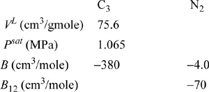
15.13. A vessel initially containing propane at 30°C is connected to a nitrogen cylinder, and the pressure is isothermally increased to 2.07 MPa. What is the mole fraction of propane in the vapor phase? You may assume that the solubility of N2 in propane is small enough that the liquid phase may be considered pure propane. Calculate using the following data at 30°C.
15.14. A 50-mol% mixture of propane(1) + n-butane(2) enters a flash drum at 37°C. If the flash drum is maintained at 0.6 MPa, what fraction of the feed exits as a liquid? What are the compositions of the phases exiting the flash drum? Work the problem the following two ways.
a. Use Raoult’s law.
b. Assume ideal mixtures of vapor and liquid (Ki is independent of composition).

15.15. A mixture containing 5 mol% ethane, 57 mol% propane, and 38 mol% n-butane is to be processed in a natural gas plant. Estimate the bubble-point pressure, the liquid composition, and K-ratios of the coexisting vapor for this mixture at all pressures above 1 bar at which two phases exist. Set kij = 0. Use the shortcut K-ratio method. Plot ln P versus 1/T for your results. What does this plot look like? Plot log Ki versus 1/T. What values do the Ki approach?
15.16. Vapor-liquid equilibria are usually expressed in terms of K factors in petroleum technology. Use the Peng-Robinson equation to estimate the values for methane and benzene in the benzene + methane system with equimolar feed at 300 K and a total pressure of 30 bar and compare to the estimates based on the shortcut K-ratio method.
15.17. Benzene and ethanol form azeotropic mixtures. Prepare a y-x and a P-x-y diagram for the benzene + ethanol system at 45°C assuming the Peng-Robinson model and using the experimental pressure at xE = 0.415 to estimate k12. Compare the results with the experimental data of Brown and Smith cited in problem 10.2.
15.18. A storage tank is known to contain the following mixture at 45°C and 15 bar on a mole basis: 31% ethane, 34% propane, 21% n-butane, 14% i-butane. What is the composition of the coexisting vapor and liquid phases, and what fraction of the molar contents of the tank is liquid?
15.19. The CRC Handbook lists the atmospheric pressure azeotrope for ethanol + methylethylketone at 74.8°C and 34 wt% ethanol. Estimate the value of the Peng-Robinson k12 for this system.
15.20. The CRC Handbook lists the atmospheric pressure azeotrope for methanol + toluene at 63.7°C and 72 wt% methanol. Estimate the value of the Peng-Robinson k12 for this system.
15.21. Use the Peng-Robinson equation for the ethane/heptane system.
a. Calculate the P-x-y diagram at 283 K and 373 K. Use k12 = 0. Plot the results.
b. Based on a comparison of your diagrams with what would be predicted by Raoult’s law at 283 K, does this system have positive or negative deviations from Raoult’s law?
15.22. One mol of n-butane and one mol of n-pentane are charged into a container. The container is heated to 90°C where the pressure reads 7 bar. Determine the quantities and compositions of the phases in the container.
15.23. Consider a mixture of 50 mol% n-pentane and 50 mol% n-butane at 15 bar.
a. What is the dew temperature? What is the composition of the first drop of liquid?
b. At what temperature is the vapor completely condensed if the pressure is maintained at 15 bar? What is the composition of the last drop of vapor?
15.24. LPG gas is a fuel source used in areas without natural gas lines. Assume that LPG may be modeled as a mixture of propane and n-butane. Since the pressure of the LPG tank varies with temperature, there are safety and practical operating conditions that must be met. Suppose the desired maximum pressure is 0.7 MPa, and the lower limit on desired operation is 0.2 MPa. Assume that the maximum summertime tank temperature is 50°C, and that the minimum wintertime temperature is –10°C. [Hint: On a mass basis, the mass of vapor within the tank is negligible relative to the mass of liquid after the tank is filled.]
a. What is the upper limit (mole fraction) of propane for summertime propane content?
b. What is the lowest wintertime pressure for this composition from part (a)?
c. What is the lower limit (mole fraction) of propane for wintertime propane content?
d. What is the highest summertime pressure for this composition from part (b)?
15.25. The kij for the pentane + acetone system has been fitted to a single point in problem P15.6. Generate a P-x-y diagram at 312.75 K.
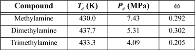
15.26. The synthesis of methylamine, dimethylamine, and trimethylamine from methanol and ammonia results in a separation train involving excess ammonia and converted amines. Use the Peng-Robinson equation with kij = 0 to predict whether methylamine + dimethylamine, methylamine + trimethylamine, or dimethylamine + trimethylamine would form an azeotrope at 2 bar. Would the azeotropic behavior identified above be altered by raising the pressure to 20 bar? Locate experimental data relating to these systems in the library. How do your predictions compare to the experimental data?
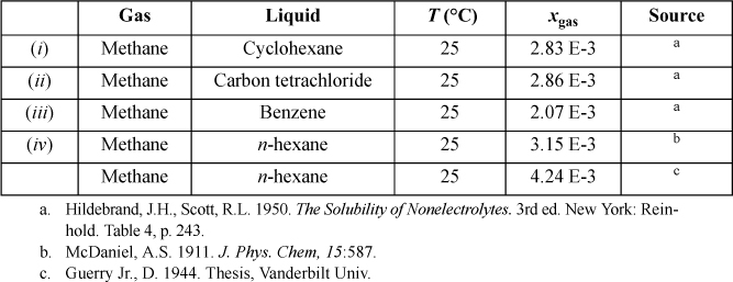
15.27. For the gas/solvent systems below, we refer to the “gas” as the low molecular weight component. Experimental solubilities of light gases in liquid hydrocarbons are tabulated below. The partial pressure of the light gas is 1.013 bar partial pressure. Do the following for each assigned system.
a. Estimate the partial pressure of the liquid hydrocarbon by calculating the pure component vapor pressure via the Peng-Robinson equation, and by subsequently applying Raoult’s law for that component.
b. Estimate the total pressure and vapor composition using the results of step (a).
c. Use the Peng-Robinson equation with kij = 0 to calculate the vapor and liquid compositions that result in 1.013 bar partial pressure of the light gas and compare the pressure and gas phase composition with steps (a) and (b).
d. Henry’s law asserts that ![]() , when xi is near zero, and hi is the Henry’s law constant. Calculate the Henry’s law constant from the calculations of part (c).
, when xi is near zero, and hi is the Henry’s law constant. Calculate the Henry’s law constant from the calculations of part (c).
e. Calculate the solubility expected at 2 bar partial pressure of light gas by using Henry’s law as well as by the Peng-Robinson equation and comment on the results.
15.28. Estimate the solubility of carbon dioxide in toluene at 25°C and 1 bar of CO2 partial pressure using the Peng-Robinson equation with a zero binary interaction parameter. The techniques of problem 15.27 may be helpful.
15.29. Oxygen dissolved in liquid solvents may present problems during use of the solvents.
a. Using the Peng-Robinson equation and the techniques introduced in problem 15.27, estimate the solubility of oxygen in n-hexane at an oxygen partial pressure of 0.21 bar.
b. From the above results, estimate the Henry’s law constant.
15.30. Estimate the solubility of ethylene in n-octane at 1 bar partial pressure of ethylene and 25°C. The techniques of problem 15.27 may be helpful. Does the system follow Henry’s law up to an ethylene partial pressure of 3 bar at this temperature? Provide the vapor compositions and total pressures for the above states.
15.31. Henry’s law asserts that ![]() , when xi is near zero, and hi is the Henry’s law constant. Gases at high reduced temperatures can exhibit peculiar trends in their Henry’s law constants. Use the Peng-Robinson equation to predict the Henry’s law constant for hydrogen in decalin at T = [300 K, 600 K]. Plot the results as a function of temperature and compare to the prediction from the shortcut prediction. Describe in words the behavior that you observe.
, when xi is near zero, and hi is the Henry’s law constant. Gases at high reduced temperatures can exhibit peculiar trends in their Henry’s law constants. Use the Peng-Robinson equation to predict the Henry’s law constant for hydrogen in decalin at T = [300 K, 600 K]. Plot the results as a function of temperature and compare to the prediction from the shortcut prediction. Describe in words the behavior that you observe.
15.32. A gas mixture follows the equation of state
where b is the size parameter, ![]() , and a is the energetic parameter,
, and a is the energetic parameter, ![]() . Derive the formula for the partial molar enthalpy for component 1 in a binary mixture, where the reference state for both components is the ideal gas state of TR, PR, and the pure component parameters are temperature-independent.
. Derive the formula for the partial molar enthalpy for component 1 in a binary mixture, where the reference state for both components is the ideal gas state of TR, PR, and the pure component parameters are temperature-independent.
15.33. The procedure for calculation of the residual enthalpy for a pure gas is shown in Example 8.5 on page 316. Now consider the residual enthalpy for a binary gas mixture. For this calculation, it is necessary to determine da/dT for the mixture.
a. Write the form of this derivative for a binary mixture in terms of da1/dT and da2/dT based on the conventional quadratic mixing rule and geometric mean combining rule with a nonzero kij.
b. Provide the expression for the residual enthalpy for a binary mixture that follows the Peng-Robinson equation.
c. A mixture of 50 mol% CO2 and 50 mol% N2 enters a valve at 7 MPa and 40°C. It exits the valve at 0.1013 MPa. Explain how you would determine whether CO2 precipitates, and if so, whether it would be a liquid or solid.
15.34. A gaseous mixture of 30 mol% CO2 and 70 mol% CH4 enters a valve at 70 bar and 40°C and exits at 5.3 bar. Does any CO2 condense? Assume that the mixture follows the virial equation. Assume that any liquid that forms is pure CO2. The vapor pressure of CO2 may be estimated by the shortcut vapor pressure equation. CO2 sublimes at 0.1013 MPa and –78.8°C, although freezing is less likely.
15.35. The vapor-liquid equilibria for the system acetic acid(1) + acetone(2) needs to be characterized in order to simulate an acetic anhydride production process. Experimental data for this system at 760 mmHg have been reported by Othmer (1943)4 as summarized below. Use the data at the equimolar composition to determine a value for the binary interaction parameter of the Peng-Robinson equation. Based on the value you determine for the binary interaction parameter, determine the percent errors in the Peng-Robinson prediction for this system at a mole fraction of x(1) = 0.3.

15.36. A mixture of methane and ethylene exists as a single gas phase in a spherical tank (10 m3) on the grounds of a refinery. The mixture is at 298 K and 1 MPa. It is a spring day, and the atmospheric temperature is also 298 K. The mole fraction of ethylene is 20 mol%. Your supervisor wants to draw off gas quickly from the bottom of the tank until the pressure is 0.5 MPa. However, being astute, you suggest that depressurization will cause the temperature to fall, and might cause condensation.
a. Provide a method to calculate the change in temperature with respect to moles removed or tank pressure valid up until condensation starts. Assume the depressurization is adiabatic and reversible. Provide relations to find answers, and ensure that enough equations are provided to calculate numerical values for all variables, but you do not need to calculate a final number.
b. Would the answer in part (a) provide an upper or lower limit to the expected temperature?
c. Outline how you could find the P, T, n of the tank where condensation starts. Provide relations to find answers, and ensure that enough equations are provided to calculate numerical values for all variables, but you do not need to calculate a final number.
a. At 298 K, butane follows the equation of state: P(V – b) = RT at moderate pressures, where b is a function of temperature. Calculate the fugacity for butane at a temperature of 298 K and a pressure of 1 MPa. At this temperature, b = –732 cm3/mol.
b. Pentane follows the same equation of state with b = –1195 cm3/mol at 298 K. In a mixture, b follows the mixing rule: ![]() where b12 = –928 cm3/mol. Calculate the fugacity of butane in a 20 mol% concentration in pentane at 298 K and 1 MPa, assuming the mixture is an ideal solution.
where b12 = –928 cm3/mol. Calculate the fugacity of butane in a 20 mol% concentration in pentane at 298 K and 1 MPa, assuming the mixture is an ideal solution.
15.38. The Soave equation of state is:
where the mixing and combining rules are given by Eqns. 15.8 and 15.9. Develop an expression for the fugacity coefficient and compare it to the expression given by Soave (1972. Chem. Eng. Sci. 27:1197).
15.39. The following equation of state has been proposed for hard-sphere mixtures:
where ![]()
Derive an expression for the fugacity coefficient.
15.40. The equation of state below has been suggested. Derive the expression for the fugacity coefficient.
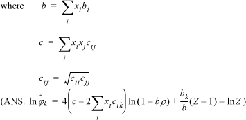
Z = 1 + 4cρ/(1 – bρ)
15.41. The following free energy model has been suggested as part of a new equation of state for mixtures. Derive the expression for the fugacity coefficient of component 1.